Prerequisites:
Firm grounding in the Basics of Data Structures
Recursion
Algorithmic complexity
Welcome to a festive new installment of Algosaurus! ‘Tis the season of Christmas trees and holly, so today, we’ll be talking about a special tree for the occasion, called the Segment Tree.
Mind you, this isn’t such an easy-to-understand data structure, but is indeed one of the most elegant and useful ones out there. It’s a long-ish post, so we’ve kept a few checkpoints to keep track of where you are:
Peep the duck and her family is decorating their Christmas tree with shiny new baubles today.

She has some mild OCD, so she divides her tree into different sections and wants to calculate the number of baubles between any 2 sections. At the same time, her babies keep adding baubles to any section whenever they like.

She decides to keep track of the number of baubles in each section through an array A.

Let’s call the operation of finding the number of baubles between section x and section y, query x y; the operation of Peep’s babies adding y baubles to section x, add x y
Basically, query x y asks the sum of the values  to
to  , and
, and add x y asks to add the value  at the index
  .
.

Of course, that doesn’t sound hard at all! Peep can just iterate from  to
to  each time she decides to query, and updates are even simpler, she can just set
  .
.
Let us analyze her solution. She takes  time per query, and
  time per update.
But what if there are a lot of queries? We’d need to iterate over a range multiple times, so that doesn’t sound so good in terms of complexity.
Enter, the prefix sum array. Instead of merely storing A, we store an array B, which stores the *cumulative sum* up till that index of A, like so:

Despite the super fancy name and definition, prefix sums are simple creatures. Calculating them is easy-peasy.
def prefix_calc(A):
    B = []
    curr = 0
    for i in A:
        curr += i
        B.append(curr)
    return B
Note how we’re calculating each element of B in , for a total run-time of . Now, we can answer queries in , by simply returning  .
.
Yay! But wait, what happens when her babies add some new baubles, ie. we get an update?
For every update in A, we need to update the elements in B as well, since the sum changes accordingly. We need to run over elements of B, so updates are .

When her tree is tiny, she can still afford to count the baubles individually. But what if she has to decorate the Christmas tree at Rockefeller Center?

Hmm, looks like we need to think a bit about this.
So the prefix sum is very quick for queries, and the generic array is very quick for updates. An important question to ask at this point is, why?
It’s because in the prefix sum, any given query can be broken into 2 values in the structure we have. And in the generic array, each update is to change a single element. These are all constant values which don’t change with the *indexes* of the queries or the updates.
What if we found a middle ground, one that does both things reasonably quickly?
The beauty of the prefix sum array B, is that it functions using a running sum broken into intervals, but the downside is that you have to update every element of B when even a single element of the original array A is updated.
In other words, the cumulative sum of every element up till the given index in B, is strongly dependent on the elements of array A. We need to decouple intervals from updates as much as we can, because we’re lazy and don’t want to update our interval values unless we *really* need to.
Why? Because that speeds up updates of course! Let’s play around with array B a bit.

Hmm, this isn’t particularly helpful. We’ll still have to loop over all the elements in A to produce this value, in case of an update. Let’s split this into 2 and see what happens.

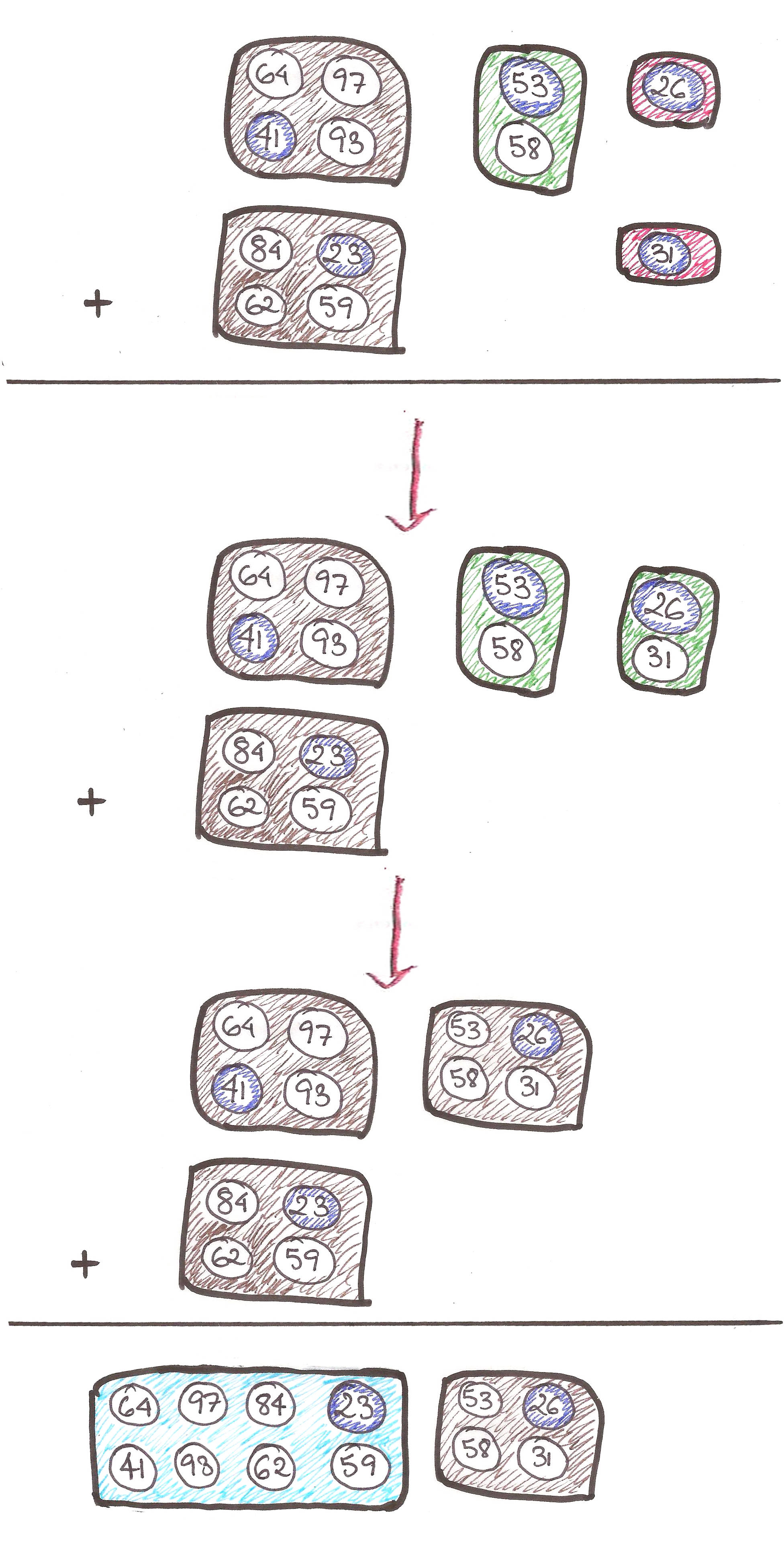
Slightly better. If any update happens between indices 1…4 of A, we don’t have to calculate the running sum of indices 5…8 anymore. We can simply recalculate the running sum of 1…4 and add to it the run sum of 5..8.

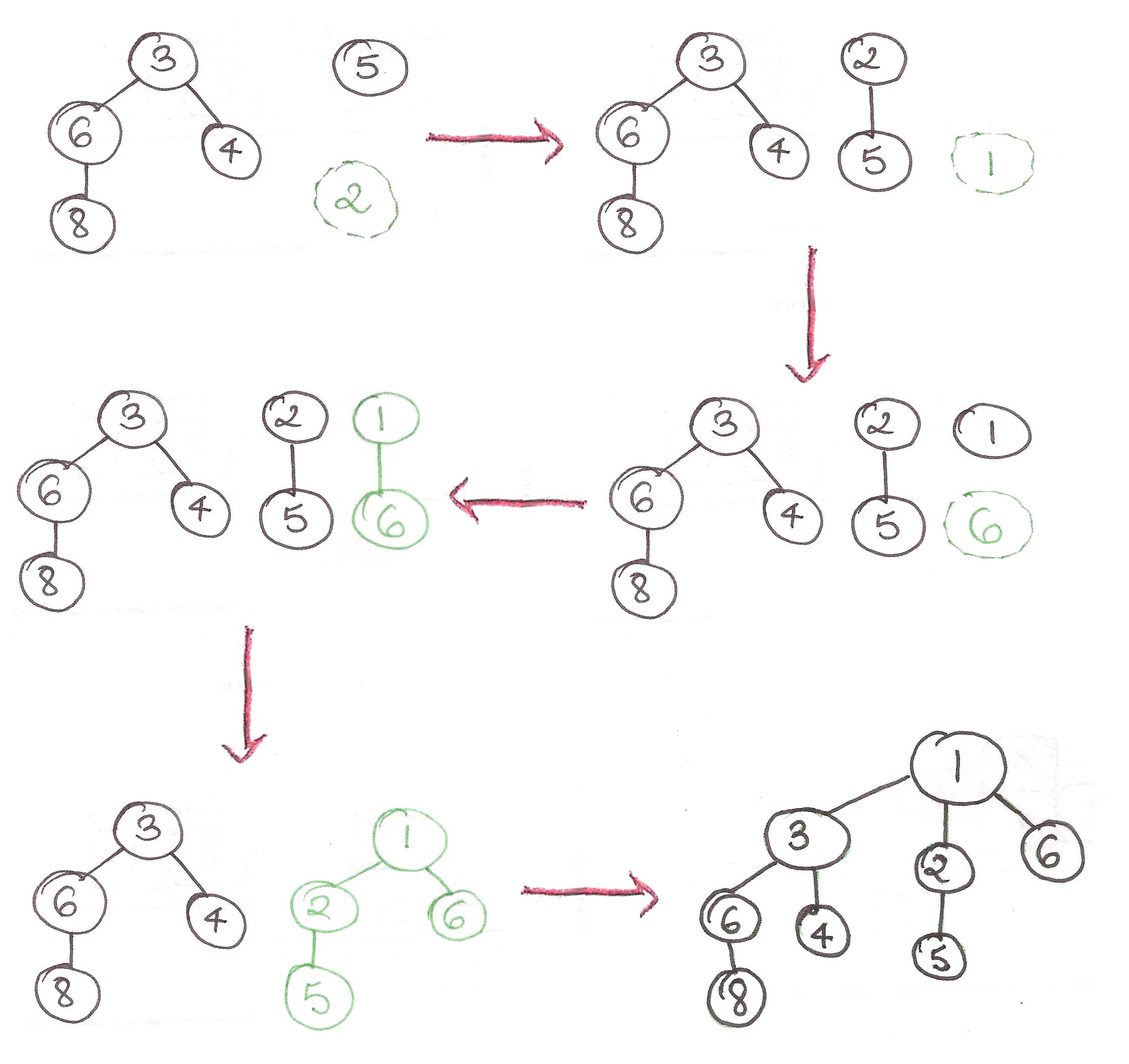
Now we’re talking. Any change in the interval, say, 3…4 won’t affect the run sums of 1..2 and 5…8. Simply recalculate the run sum of 3…4 and let the change in 3…4 ‘percolate’ to 1…4 and then to 1…8.
And finally…

The last level of ‘decoupling’ updates from intervals, and reducing the dependence of pre-calculated run sums from the elements of A. Any change in a single element won’t affect the rest of the elements.
This is called a segment tree.
Since this kind of structure is formed by the *union* of intervals or segments, it supports any function which supports the union operator.
That means Peep can find the greatest number of baubles between any 2 sections as well! (Since max supports the union operator as well, ie. if max(a, b) = a and max(c, d) = d, then max(a, b, c, d) = max(a, d))

Why is this nice? Note that each index in the original array appears in  nodes (one on each level), which is
  . This means that if we change the value of a single element, nodes in the segment tree change. Which implies that we can do updates quickly.
Note that any interval can be expressed as a union of some nodes of the tree. As an example look at the nodes we need for  .
.

We claim that any interval can be represented by nodes in the tree, so we can conceivably do queries quickly too. We’ll prove this after talking about the query function itself right here, so stay put!
Let’s now try to count the number of nodes. There’s  leaves (leaves are nodes with no children),
  nodes in the level above,
  above that, and so on, until
  . This gives us the sum
  , which sums to
Summing up, this means we can do updates and queries in , in space.

Let’s concretely make our functions now.

Now, for each node indexed  , if isn’t a leaf node, its children are indexed
  and
and  . These observations suffice to describe a
 build method, with which we can initialize the tree. Note that we’ve used an array of size  to represent the tree. This is necessary because of the full binary-heap like representation of the segment tree we’re using.
max_N = (1 << 20) #This is the maximum size of array our tree will support
seg = [0] * (4 * max_N) #Initialises the ’tree’ to all zeroes.

def build(someList, v, L, R):
    global seg
    if (L == R):
        seg[v] = someList[L]
    else:
        mid = (L + R) / 2 #Integer division is equivalent to flooring.
        build(someList, 2 * v, L, mid)
        build(someList, 2 * v + 1, mid + 1, R)
        seg[v] = seg[2 * v] + seg[2 * v + 1]
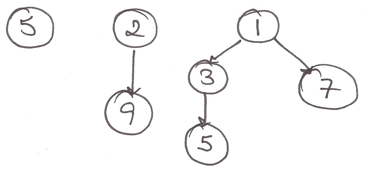
For the update procedure, the simplest way is to travel down to the lowest level, make the necessary update, and let it travel back up the tree as we add the left and right children for every node.
Let’s use an example!

This procedure can be described very cutely with a recursive function.
def update(v, L, R, x, y):
    global seg
    if (L <= x <= R): #the index to be updated is part of this node
        if (L == R): #this is a leaf node
            seg[v] += y
        else:
            mid = (L + R) / 2
            update(2 * v, L, mid, x, y)
            update(2 * v + 1, mid + 1, R, x, y)

            #update node using new values of children
            seg[v] = seg[2 * v] + seg[2 * v + 1]
Consider a query. Say that the query asks for the sum of values in the interval  . Say, further, that we are on node , which represents the interval
  . There are three possibilities:
1. and do not intersect. In this case, we are not interested in the value of this node.
2.  . In this case, we will use the value of the node as is.
3. There is a part of , which resides outside . Here, it makes sense to examine the children of , to find the intervals that fit better, or not at all (see cases 1 and 2).

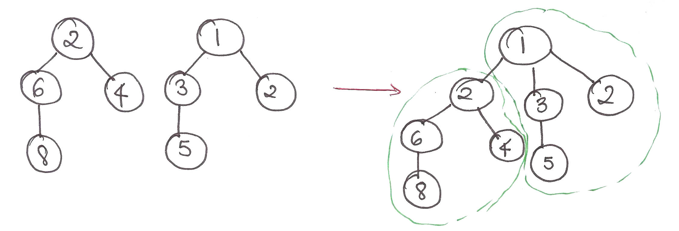
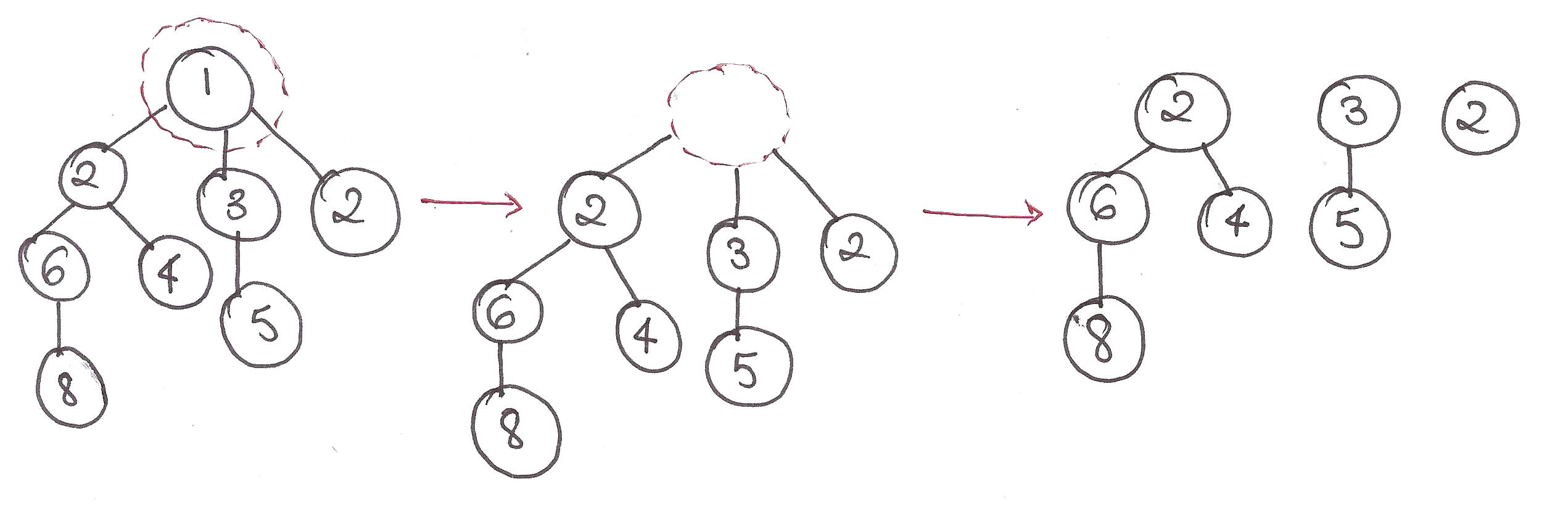
Let’s look at a concrete example!

So the answer to the query is stored in run sum (or whatever you call it).
This can be represented in a recursive method as follows.
def query(v, L, R, x, y):
    if (R < x or y < L):
        #case 1
        return 0
    elif (x <= L <= R <= y):
        #case 2
        return seg[v]
    else:
        #case 3
        mid = (L + R) / 2
        return query(2 * v, L, mid, x, y) + query(2 * v + 1, mid + 1, R, x, y)
We’ve put up a global list-based version and a class-based version of the segment tree code on Gist, so go check them out!
Now, some interesting stuff. Let’s say that instead of the sum function, we had some function  , which takes as input a list of values and outputs a single real number. What properties should it have so that our segment tree can support it?
We are combining intervals, in for the sum function, which gives us a runtime of per operation, so if combining intervals takes time  , then each operation is
  . So we can use this structure for any whose value of is low enough to be acceptable for the given situation.
For example, for = max function,  , so the segment tree works quickly for that.
We’ll now prove that the query function runs in for any arbitrary interval.
At the heart of the proof is the fact that the query function visits at most  nodes in each level.
We always visit the root level, and it has only node, so we have a base case. Also, let’s assume that the hypothesis holds true for all levels  .
.
Now, if we visit node on the  level, then we can visit only
  in the next (since a single node has children). Note how the function only visits continuous nodes in the next level.
If we visit , then they have only children, which means we’re still fine visiting all .
We will never visit  nodes on a level. This is because if an interval does not fit well, we visit both of its children, which implies that we never visit an odd number of nodes on a level (except on root).
If we visit nodes on a level, then by the previous argument, they must be continuous. We claim, by way of contradiction, that we will need to visit all  children from these nodes. This implies that we have case for every one of these nodes. Note, however, that if any two nodes have case , the query interval spans every node between them, which contradicts our supposition. So we’ll only visit the children of at-most nodes on this level, and hence at most nodes on the next level.
Now, since the hypothesis holds for all levels implies it holds for level  , by strong induction, it holds for every level.
Now, since there are levels, the query function will use at most  nodes per query.
And we’re done!
What if we had updates of the type:
add x y z
where one has to add  to every element between and (both inclusive)?
We could do  updates on our tree, but that would be
  , which is atrocious.
Alternatively, note that we can break up the update interval into some nodes (exactly like the query function).
But instead of reporting the sums of all the nodes which exhibit case 2, we will update all of them. If is added to every element of a node of size  , its sum increases by
  , which means we can update each node in , for an overall runtime of .
But *wait*.
The children of every non-leaf node we changed do not have the new value. What if we get a query that uses those nodes? Let’s create an additional variable for every node, called lazy, so that  stores the pending addition to node .
We’ll only do additions to a node when we *need* to use the node, since we’re lazy folks and don’t want to do any work unless we need to.

What do we mean by pending addition? The idea is that when a node falls in case 2 (from the cases we defined around the query function), we update it, and add to the pending values of its children. This adds an additional procedure to both the update and the query functions.
Before we do any work on a node, we need to apply any pending add updates, and propagate these updates to its children, by adding the updates to their lazy values.
This part is magical! All the pending changes for every update are squashed into a single update. No multiple updates are required anymore and we can make do with only 1, that too only when we need to.
Since we’re only doing an additional constant amount of work per node, everything is still !
Let’s make this procedure clearer with an example.

Now, let’s see how the lazy values come into play. Say that we call get a query 4 5.

The idea is hopefully precise enough to translate to code now. We’ve put up the code right here, so go take a look at it!
This concludes our article on segment tree. The segment tree is a rather wonderful data structure, so we hope we’ve done justice to it. As usual, we love hearing from you, so do send us your feedback at rawrr@algosaur.us!
Acknowledgements:
Stack Exchange thread on proof of time complexity of query operation on segment tree
 . That’s no good.
 time or less.


 elements into similar packets of smaller powers of 2
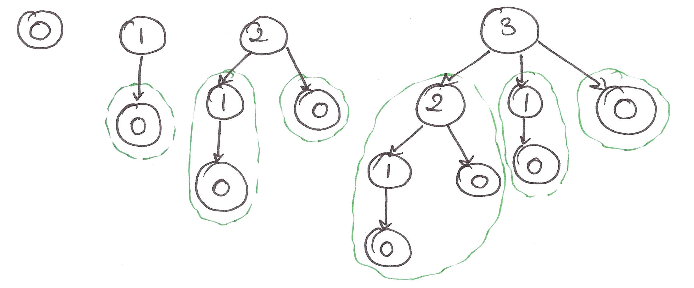
 binomial trees together at the same time.
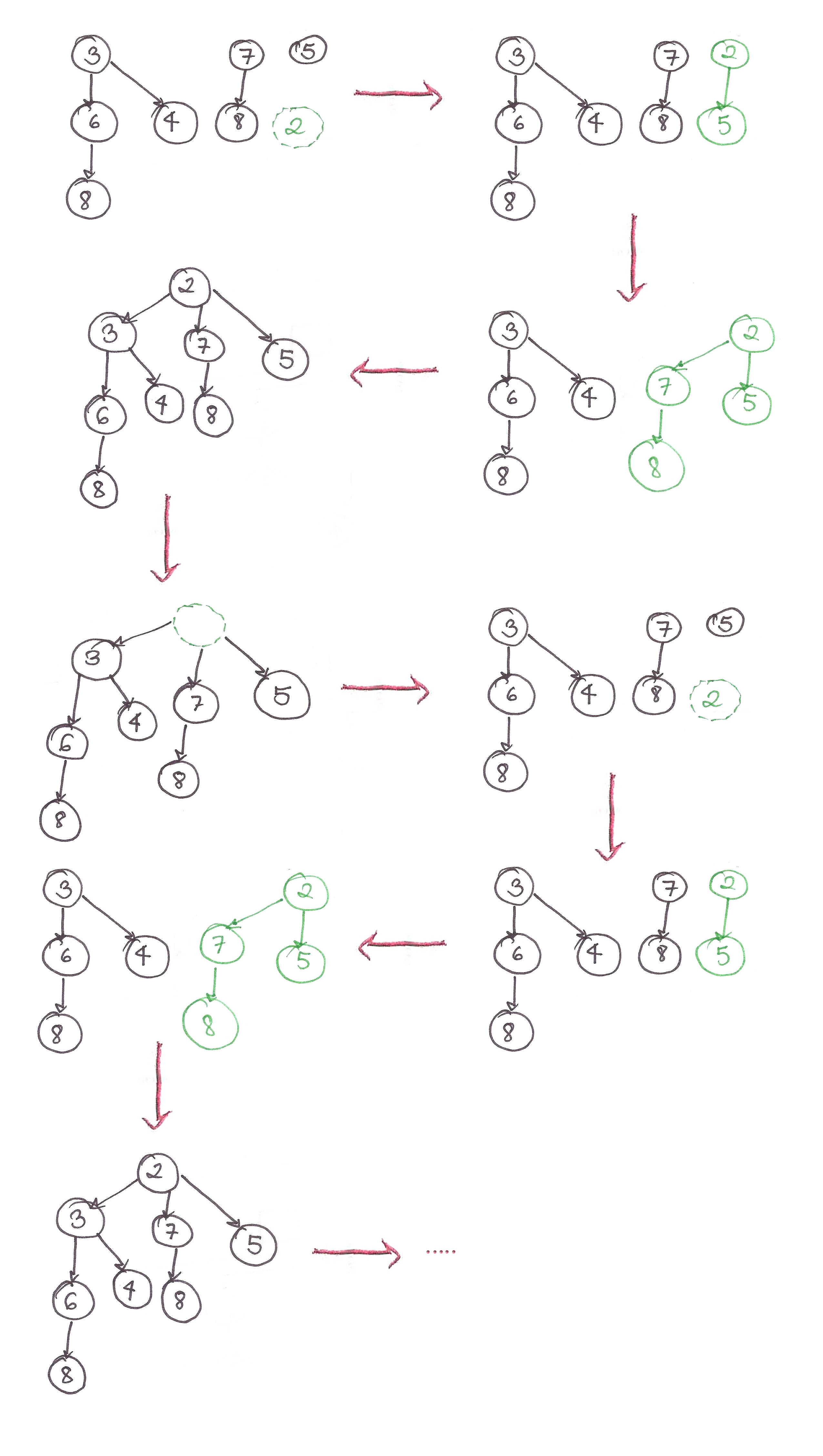
 , is
, is