Prerequisites:

• Algorithmic complexity analysis
• Arrays
• Basics of recursion

Patience Algosaurus.

Data structures by themselves aren’t all that useful, but they’re indispensable when used in specific applications, like finding the shortest path between points in a map, or finding a name in a phone book with say, a billion elements (no, binary search just doesn’t cut it sometimes!).

Oh, and did I mention that they’re used just about everywhere in software systems and competitive programming?

This time, we only have two levels and a bonus, since this is an article on just the basics of data structures. Having a Mastery level just doesn’t make sense when there’s a ridiculous number of complicated data structures.

• Introduction
• Apprenticeship
• Bonus

---

Say hello to Loopie.

Loopie enjoys playing Hockey with her family. By playing, I mean…

When the turtles are shucked into the goal, they are deposited back on top of the pile.

Evidently, Loopie’s family likes sliding on ice.

Notice how the first turtle added on the pile, is the first turtle to be ejected.

This is called a queue.

Similar to a real queue, the first element which was added to the list, will be the first element out. This is called a FIFO (First In First Out) structure.

Insertion and deletion operations?

Code:

q = []

def insert(elem):
    q.append(elem) #inserts elem into the end of the queue
    print q

def delete():
    q.pop(0) #removes 0th element of the queue
    print q

After a fun-filled afternoon playing Hockey, Loopie is making pancakes for everyone. She places all the pancakes in a similar pile.

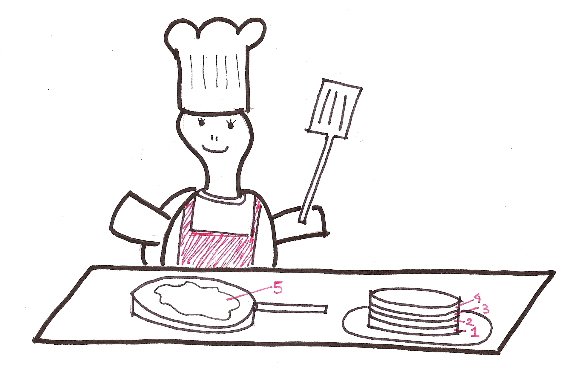
Then serves them to the family one by one.

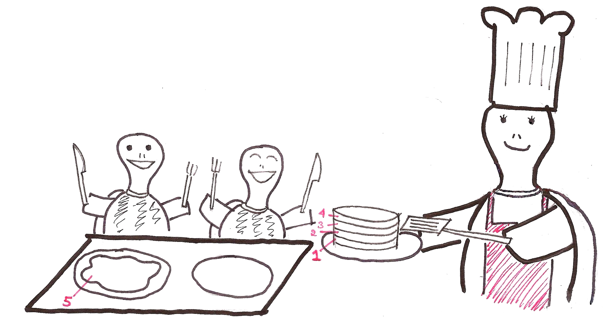
Notice how the first pancake she made, is the last one she serves.

This is called a stack.

The first element which was added to the list, will be the last one out. This is called a LIFO (Last In First Out) structure.

Insertion and deletion operations?

Code:

s = []

def push(elem): #insertion in a stack is called 'pushing' into a stack
    s.append(elem)
    print s

#deletion from a stack is called 'popping' from a stack
#pop is already a predefined function in Python for all arrays, but we'll still define it here for learning purposes as customPop()

def customPop():
    s.pop(len(s)-1)
    print s

---

Ever seen a density column?

All the items from top to bottom, are in ascending order of their densities. What happens when you drop an object of arbitrary density into the column?

It settles to the correct position on its own, due to difference in densities in the layers above and below it.

Heaps are something of that ilk.

Consider a heap like so.

A heap is a complete binary tree, meaning every parent has two children. Even though we visualize it as a heap, it is implemented through a regular array.

Also, a binary tree is always of height , where is the number of elements. By the way, in Computer Science is always considered to be by default, because we really like binary stuff.

This is a max-heap, where the fundamental heap property is that the children of any parent node, will be smaller than the parent node itself. In min-heaps, the children are always larger than the parent node.

A few basic function definitions:

global heap
global currSize

def parent(i): #returns parent index of ith index
    return i/2

def left(i): #returns left child of ith index
    return 2*i

def right(i): #returns right child of ith index
    return (2*i + 1)

Let’s tackle this part-by-part.

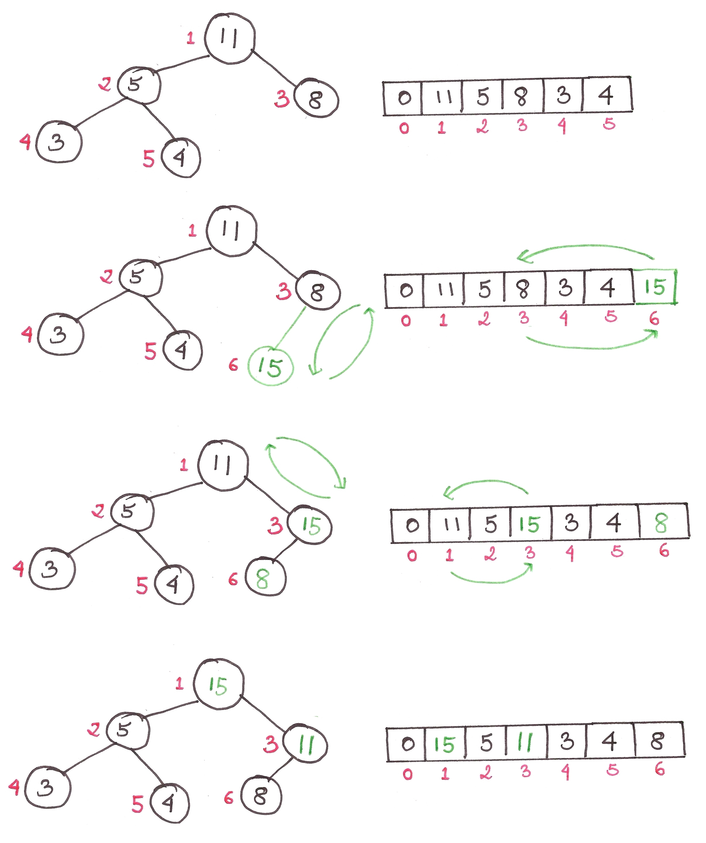
1) Inserting an element into a pre-existing heap

We first insert the element into the bottom of the heap, ie. last index in the array. Then we repeated apply the heap property on the index of the element till it reaches the appropriate position.

The algorithm is as follows:

1. Add the element to the bottom level of the heap.
2. Compare the added element with its parent; if they are in the correct order, stop.
3. If not, swap the element with its parent and return to the previous step.

Code:

def swap(a, b): #to swap a-th and b-th elements in heap
    temp = heap[a]
    heap[a] = heap[b]
    heap[b] = temp

def insert(elem):
    global currSize
    
    index = len(heap)
    heap.append(elem)
    currSize += 1
    par = parent(index)
    flag = 0
    while flag != 1:
        if index == 1: #we have reached the root of the heap
            flag = 1
        elif heap[par] > elem: #if parent index is larger than index of elem, then elem has now been inserted into the right place
            flag = 1
        else: #swaps the parent and the index itself
            swap(par, index)
            index = par
            par = parent(index)
            
    print heap

The maximum number of times this while loop can run, is the height of the tree itself, or . Hence the time complexity is .

2) Extracting the largest element from the heap

The first element of the heap is always the largest, so we just remove that and replace the top element with the bottom one. Then we restore the heap property back to the heap, through a function called maxHeapify().

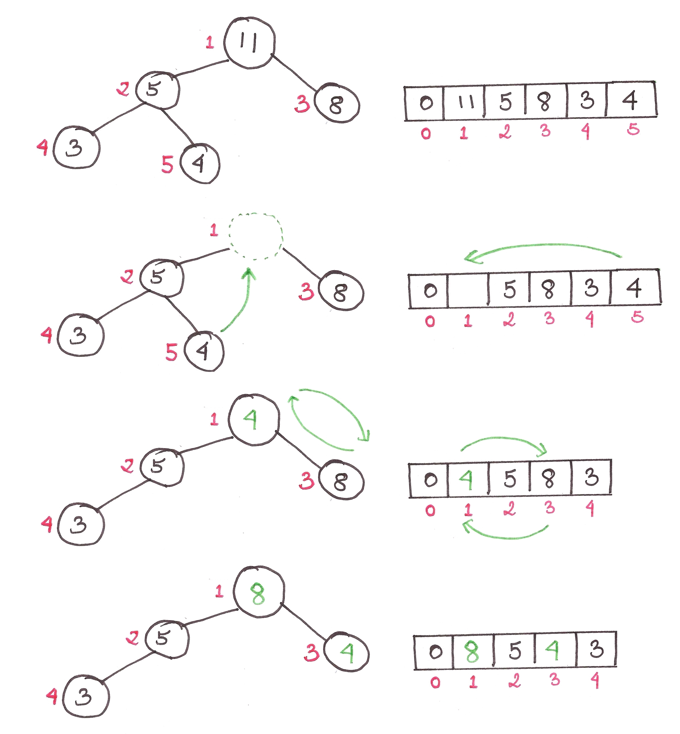
1. Replace the root of the heap with the last element on the last level.
2. Compare the new root with its children; if they are in the correct order, stop.
3. If not, swap the element with one of its children and return to Step 2. (Swap with its smaller child in a min-heap and its larger child in a max-heap.)

Code:

def extractMax():
    global currSize
    if currSize != 0:
        maxElem = heap[1]
        heap[1] = heap[currSize] #replaces root element with the last element
        heap.pop(currSize) #deletes last element present in heap
        currSize -= 1 #reduces size of heap
        maxHeapify(1)
        return maxElem

def maxHeapify(index):
    global currSize
    
    lar = index
    l = left(index)
    r = right(index)

    #print heap

    #finds the larger child of the index; if larger child exists, swaps it with the index
    if l <= currSize and heap[l] > heap[lar]:
        lar = l
    if r <= currSize and heap[r] > heap[lar]:
        lar = r
    if lar != index:
        swap(index, lar)
        maxHeapify(lar)

Again, the maximum number of times maxHeapify() can be executed, is the height of the tree itself, or . Hence the time complexity is .

3) How to make a heap out of any random array

Okay, so there’s two ways to go about it. The first way is to just repeatedly insert every element into the previously empty heap.

This is easy, but relatively inefficient. The time complexity of this comes out to be because of an function being run times.

There’s a better, more efficient way of doing this, where we simply maxHeapify() every ‘sub-heap’ from the element back to the 1st one.

This runs at complexity and it’s beyond the scope of this article to prove why. Just understand that any element past the halfway point in a binary tree, will have no children and that most of the ‘sub-heaps’ formed will be of height less than .

Code:

def buildHeap():
    global currSize
    for i in range(currSize/2, 0, -1): #third argument in range() shows increment factor, here -1
        print heap
        maxHeapify(i)
    currSize = len(heap)-1

Ah, we’ve been leading up to this question this entire time.

Heaps are used to implement an efficient sort of sort, unsurprisingly called, the Heapsort.

Unlike the sorely inefficient Insertion Sort and Bubble Sort with their measly complexities, Heapsort runs in time, beating them to the dust.

It’s not even complicated, just keep extracting the largest element from the heap till the heap is empty, placing them sequentially at back of the array where the heap is stored.

Code:

def heapSort():
    for i in range(1, len(heap)):
        print heap
        heap.insert(len(heap)-i, extractMax()) #inserting the greatest element at the back of the array
    currSize = len(heap)-1

To tie it all together, I’ve written a few lines of helper code to input elements into the heap and try out all the functions. Check it out right here. Oh, and for all the people who are acquainted with classes in Python, I’ve also written a Heap class here.

Voila! Wasn’t that easy? Here’s a partying Loopie just for coming this far.

We also use heaps in the form of priority queues to find the shortest path between points in a graph using Dijkstra’s Algorithm, but that’s a post for another day.

---

Loopie wants to teach her baby turtles how to identify shapes and colours, so she brings home a large number of pieces of different colours.

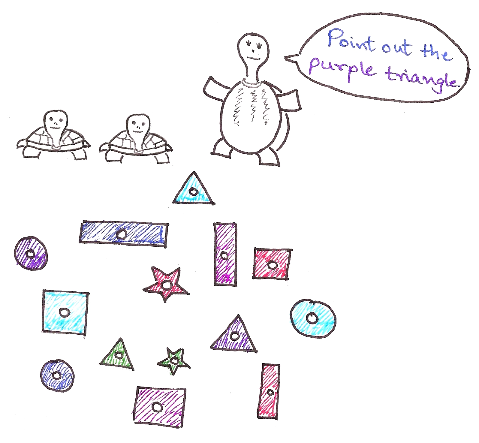
This took them a lot of time, as well as confusion.

So she gets another toy to make the process easier.
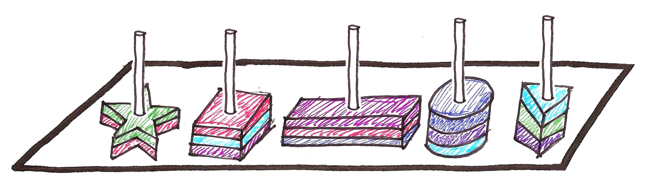This was easier because the babies already knew that the pieces were categorized according to shape. What if we labeled each of the poles as follows?

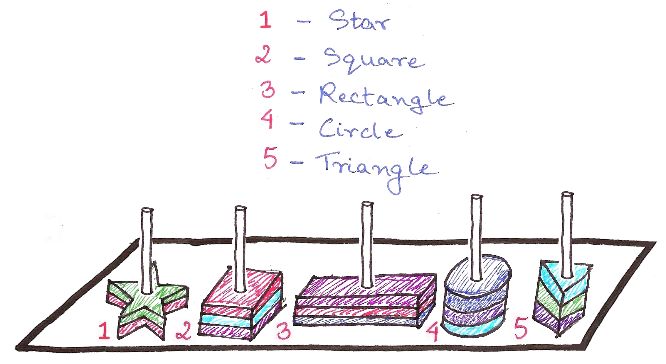
The babies would just have to check for the pole number, then look through a far smaller number of pieces on the pole.

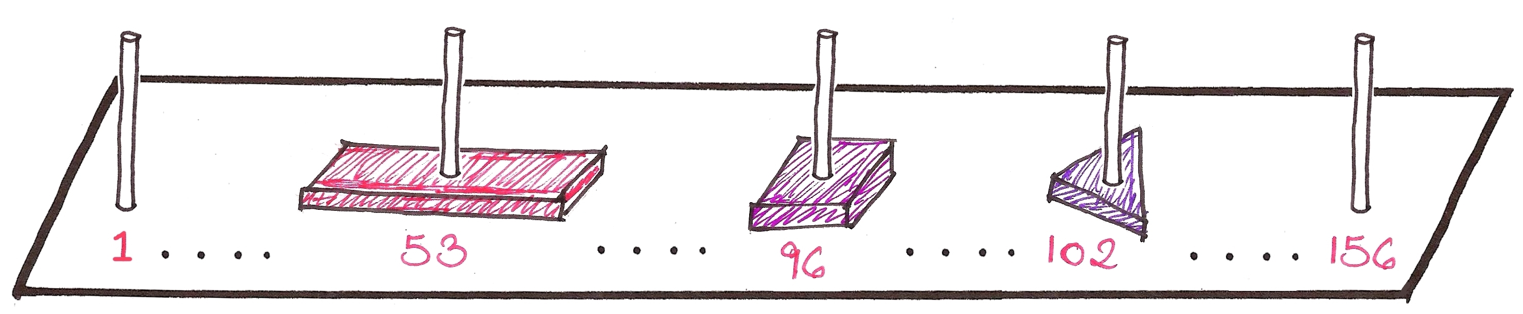
Now imagine one pole for every combination of colour and shape possible.

Let the pole number be calculated as follows:

purple triangle:
p+u+r+t+r+i = 16+21+18+20+18+9 = Pole #102

red rectangle:
r+e+d+r+e+c = 18+5+4+18+5+3 = Pole #53

etc.

We know that 6*26 = 156 combinations are possible (why?), so we’ll have 156 poles in total.

Let’s call this formula to calculate pole numbers, the hash function.

In code:

def hashFunc(piece):
    words = piece.split(" ") #splitting string into words
    colour = words[0]
    shape = words[1]
    poleNum = 0
    for i in range(0, 3):
        poleNum += ord(colour[i]) - 96
        poleNum += ord(shape[i]) - 96
    return poleNum

If we ever need to finish where ‘pink square’ is kept, we just use

hashFunc('pink square')

and check the pole number, which happens to be pole #96.

This is an example of a hash table, where the location of an element is stored in terms of a hash function. The poles here are analogous to buckets in proper terminology.

This makes time taken to search for a particular element independent of the total number of elements, ie. time.

Let this sink in. Searching in a hash table can be done in constant time.

Wow.

What if we’re searching for a ‘dreary-blue rectangle’, assuming a colour called ‘dreary-blue’ exists?

hashFunc('dreary-blue rectangle')

returns pole #53, which clashes with the pole number for ‘red rectangle’. This is called a collision.

How do we resolve it?

We use a method called separate chaining, which is a fancy way of saying every bucket consists of a list, and we simply search through the list if we ever find multiple entries.

Here, we’ll just put the dreary-blue rectangle on top of the red rectangle, and just pick either one whenever we need to.

The key in any good hash table, is to choose the appropriate hash function for the data. This is unarguably the most important thing in making a hash table, so people spend a lot of time on designing a good hash function for their purpose.

In a good hash table, no bucket should have more than 2-3 entries. If there are more, then the hashing isn’t working well, and we need to change the hash function.

Searching is independent of the number of elements for god’s sake. We can use hash tables for just about anything involving a gigantic number of elements, like database entries or phone books.

We also use hash functions in searching for strings or sub-strings in large collections of texts using the Rabin-Karp algorithm. This is useful for detecting plagiarism in academic papers by comparing them against source material. Again, a post for another day!

---

I plan on writing more on advanced data structures like Fibonacci Heaps and Segment Trees and their uses, so subscribe to Algosaurus for updates!

I hope you found this informal guide to the basics of data structures useful. If you liked it, want to insult me, or if you want to talk about dinosaurs or whatever, shoot me a mail at rawrr@algosaur.us

Acknowledgements:
Introduction to Algorithms – Cormen, Leiserson, Rivest, and Stein (pages 151 – 161)