Prerequisites:
Firm grounding in the Basics of Data Structures
Recursion
Algorithmic complexity
Hi, welcome to another installment of Algosaurus, this time on Binomial Heaps. They are a more efficient form of heaps than the simple binary heaps we looked at earlier, not to mention they have a beautiful intuition to them. Even though they aren’t frequently used, they’re still good for expanding your mind.
Let’s compare the complexities of various operations on Binary, Binomial, and Fibonacci Heaps respectively.
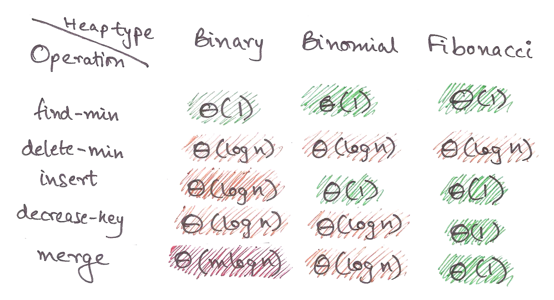
Need I say anything further?
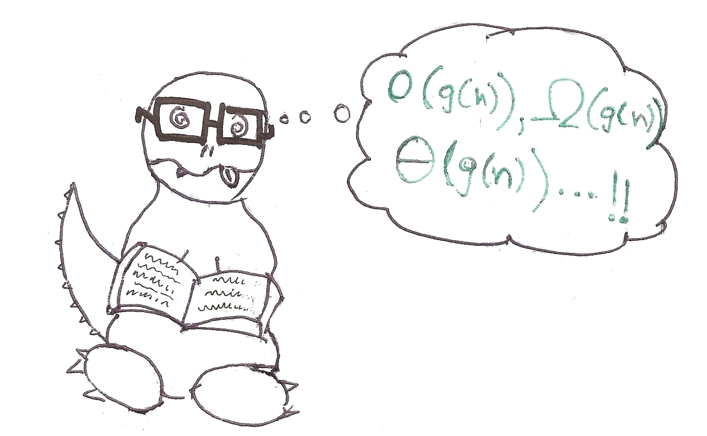
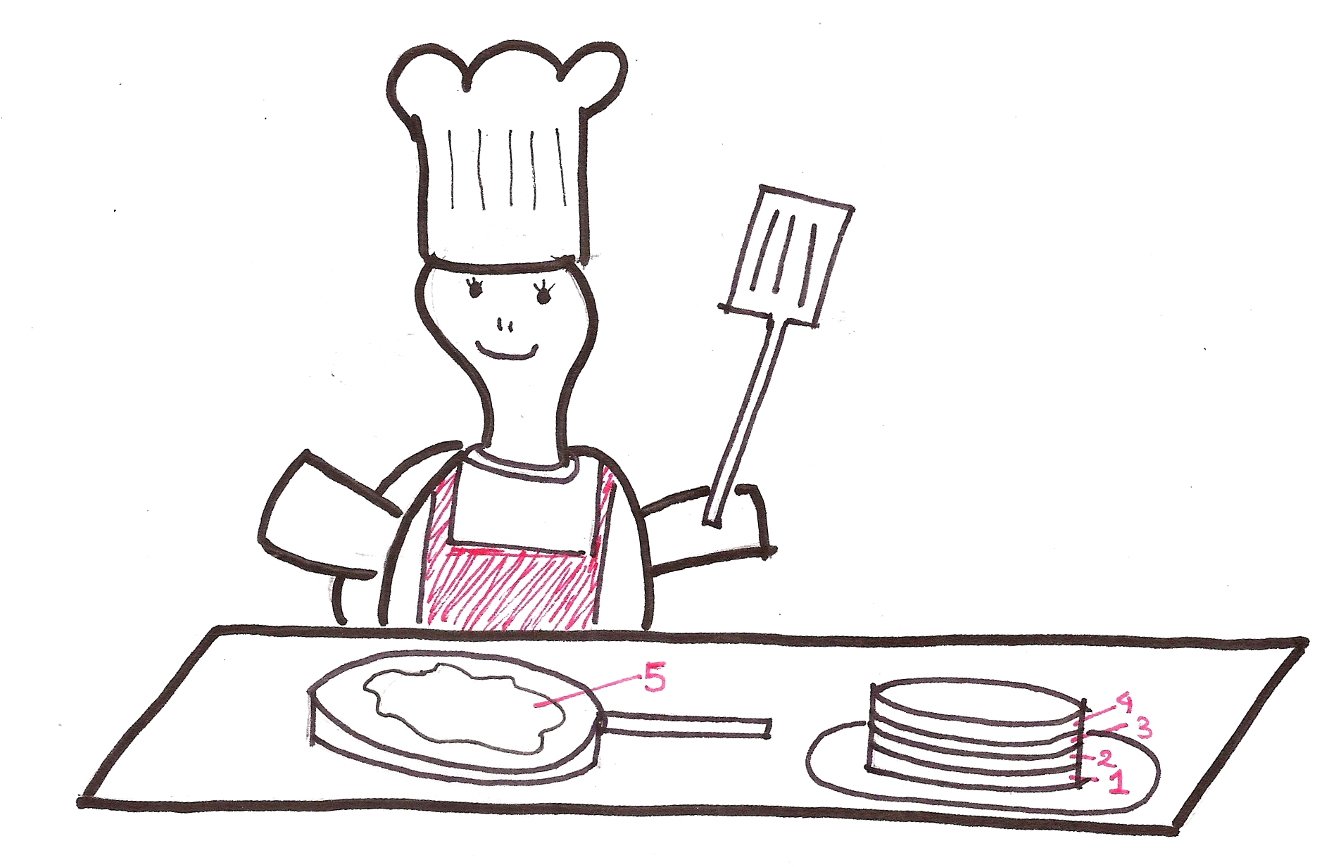
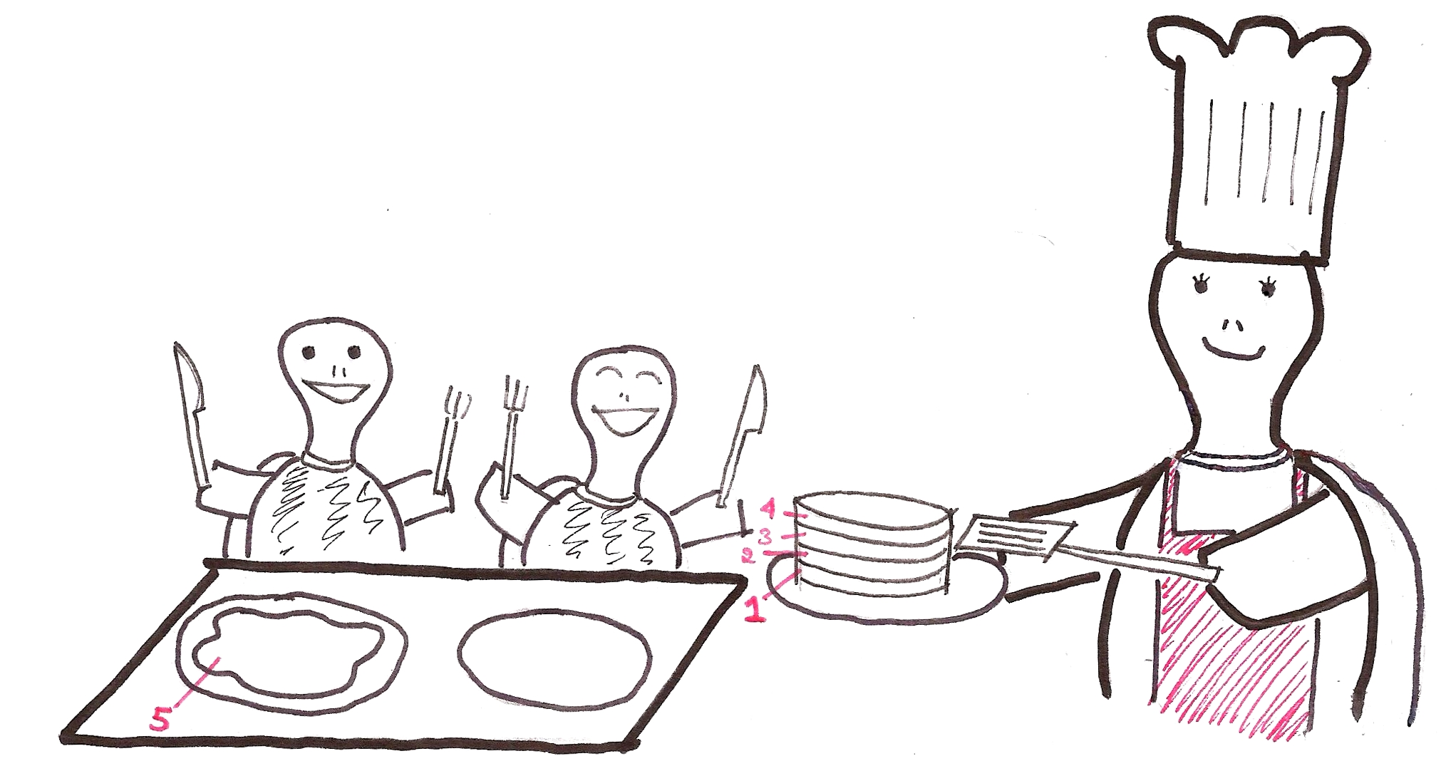
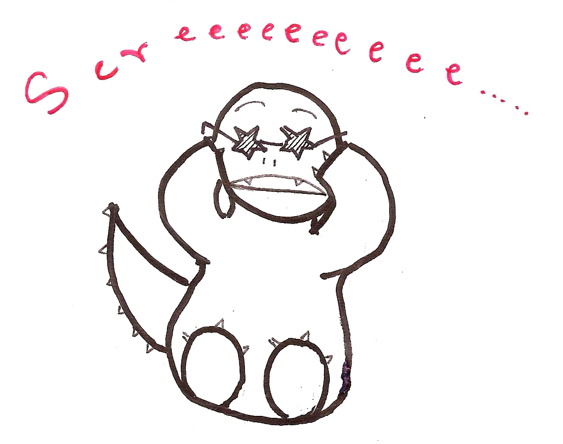
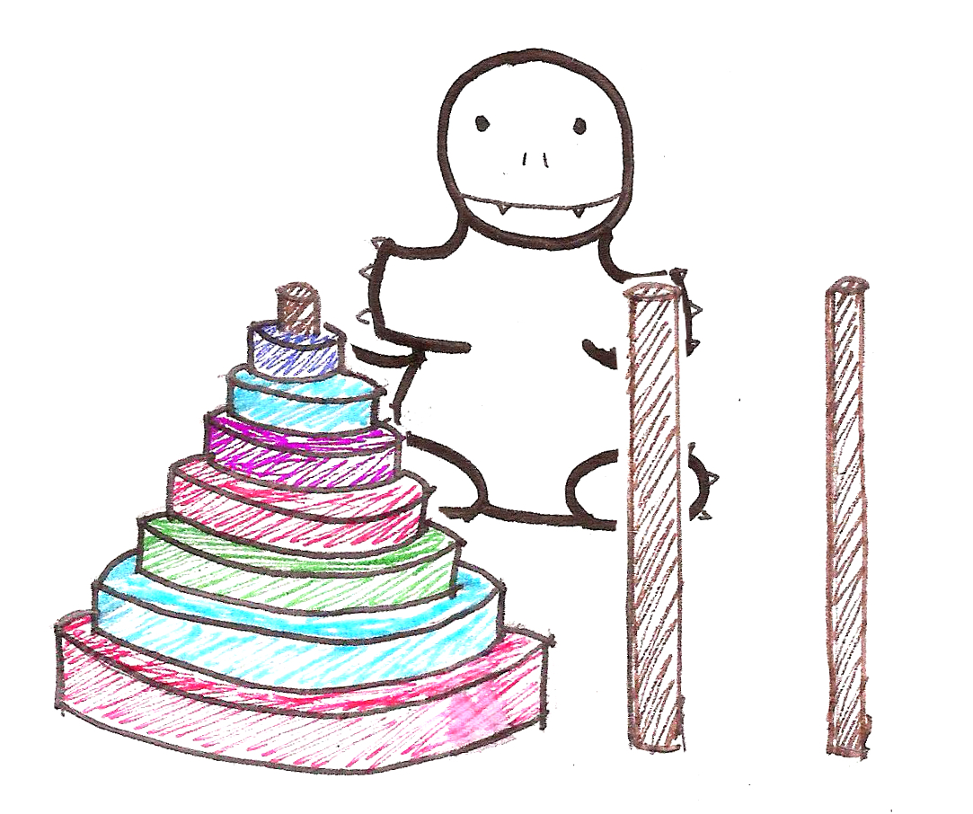
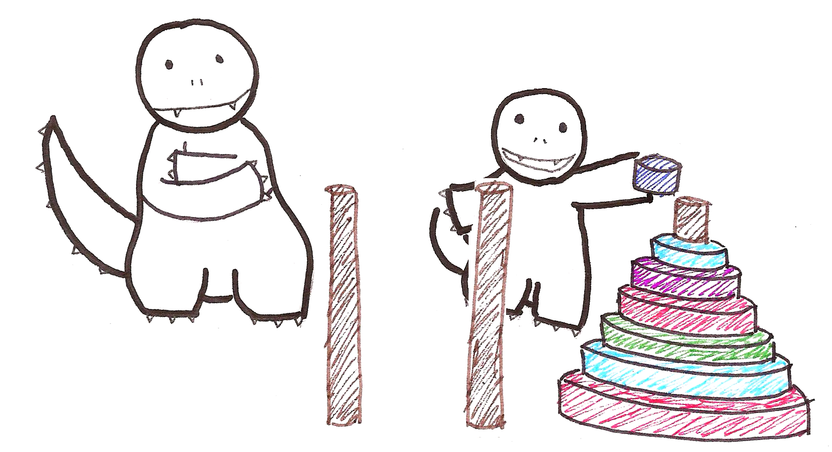
As a disclaimer, this article is definitely not aimed at beginners to programming. The Binomial Heap concept is somewhat complex and you might look like this after your first reading:

That said, let’s begin!
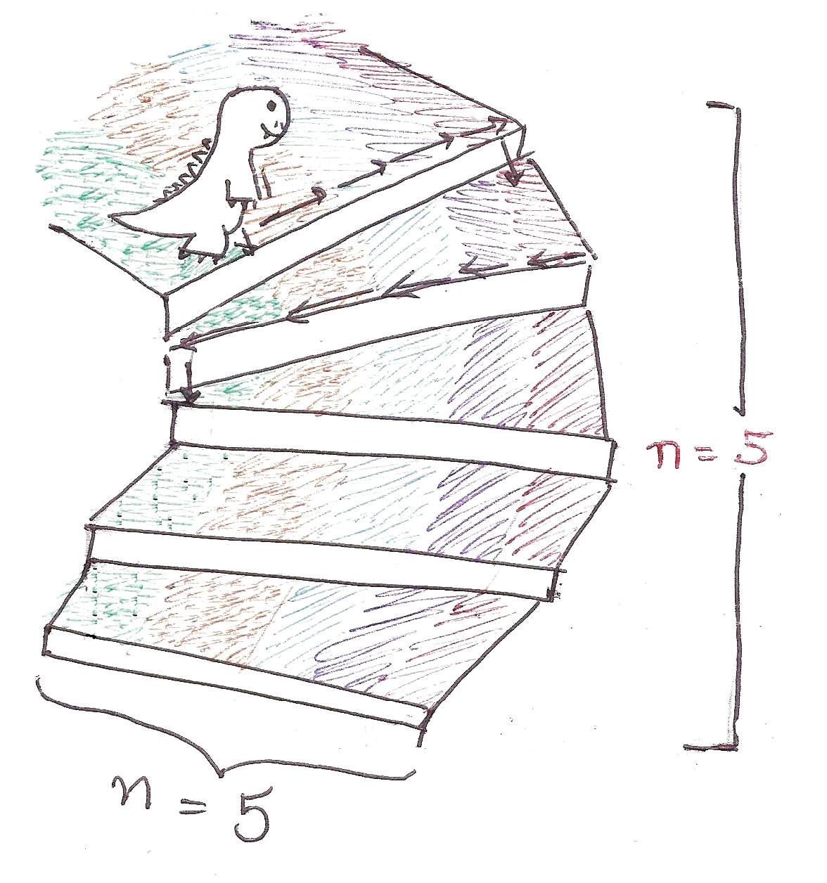
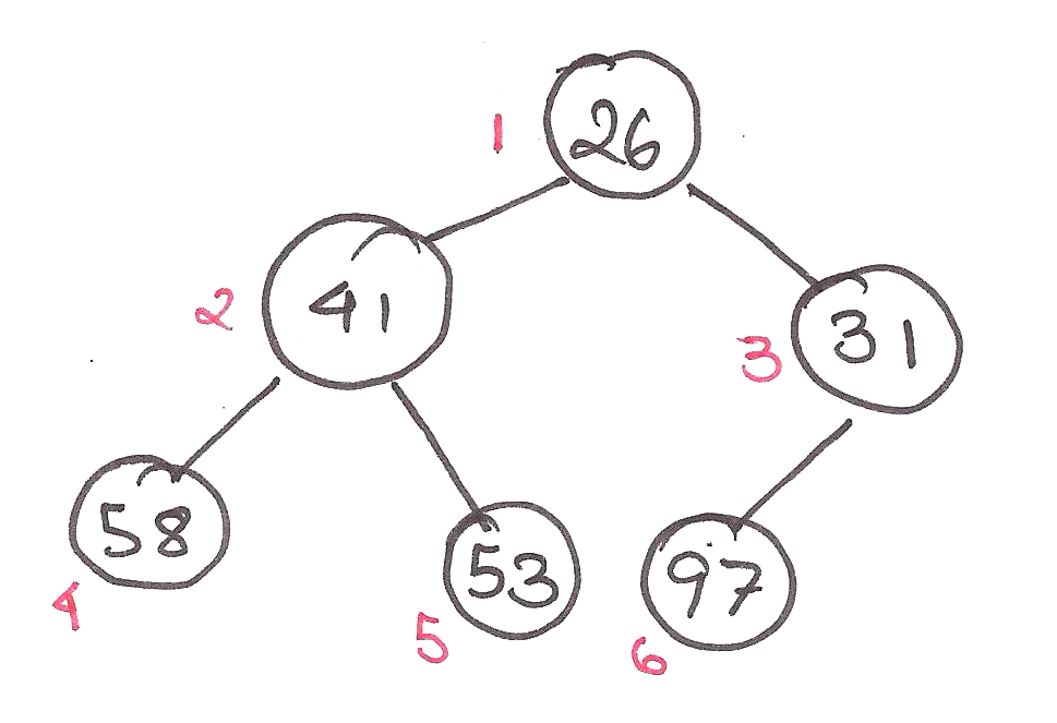
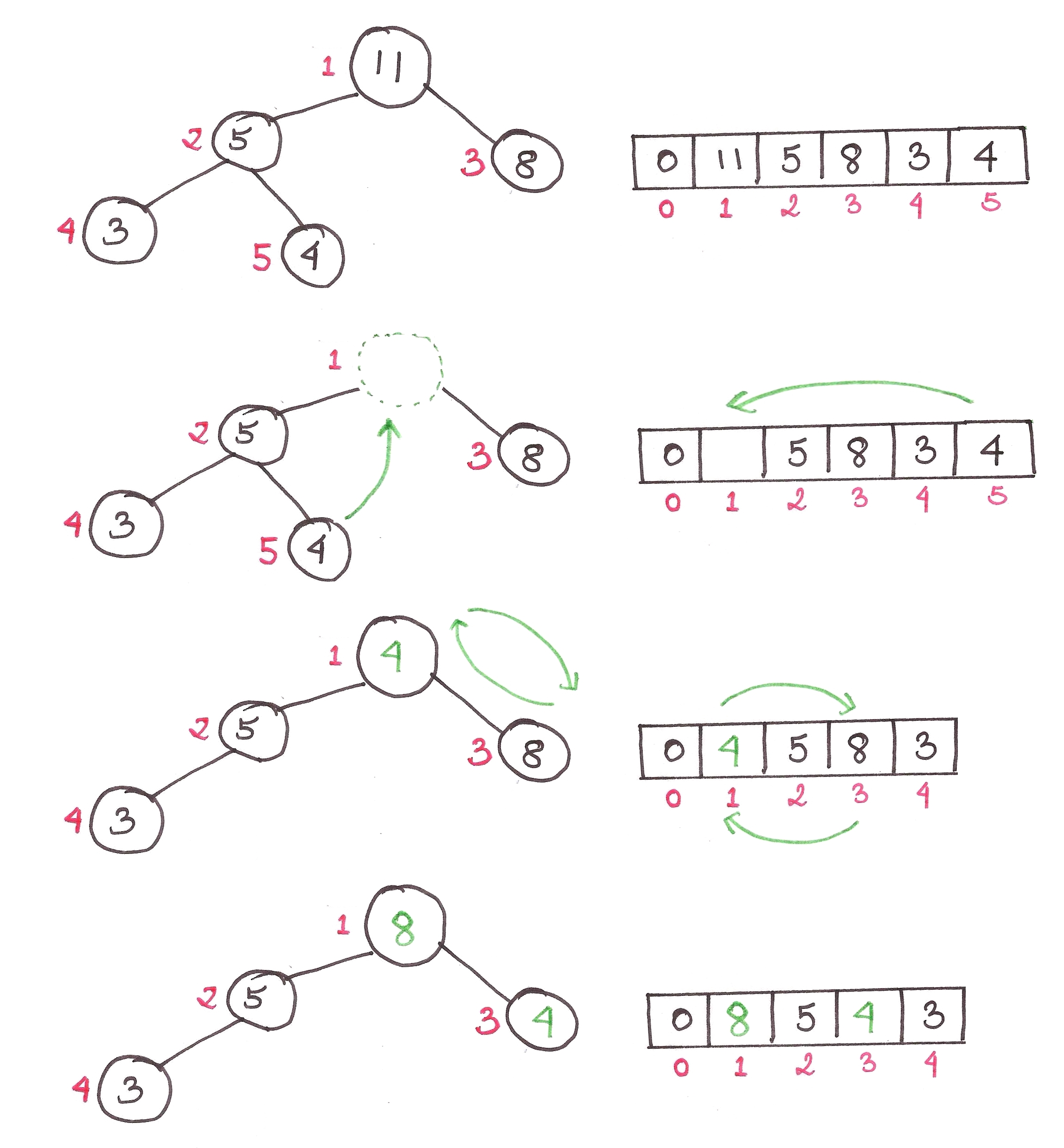
First, a quick recap of binary heaps. In my last article, I implemented binary heaps as max heaps, where the largest element was stored at the root of the tree.
Today, we’re going to show them as min-heaps, where the root element is the smallest.
Heaps were created to improve the complexity of graph algorithms like Dijkstra’s Algorithm, by executing the algorithm using a heap. Notably, binary min-heaps are used as priority queues there.
Thing is, two more operations are often used in graph algorithms.
One, merging two heaps together to form a new heap.
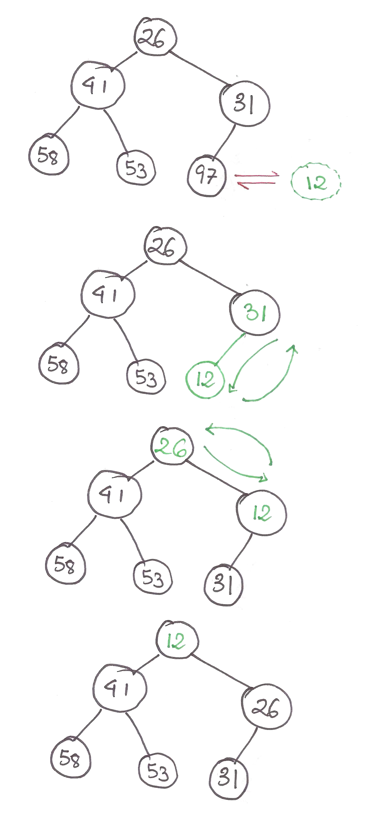
Two, decreasing the value stored in a node, called decrease-key.
There’s no easy way to merge regular binary heaps apart from reconstructing the heap from scratch, making the complexity  . That’s no good.
Once again, the time complexities for operations on binary heaps are as follows:
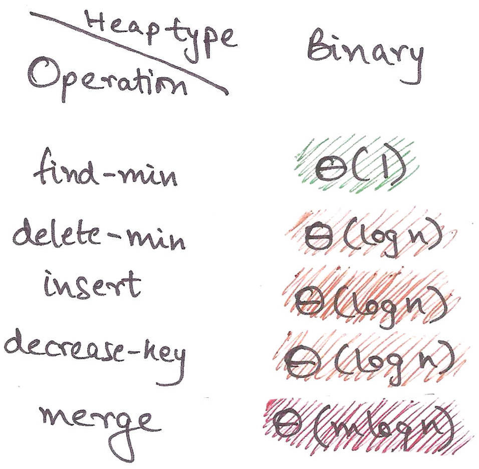
We can perform most operations in  time or less.
Question is, can we do better?
Don’t worry Algosaurus, we can make that reality.
How do we merge nicely then?
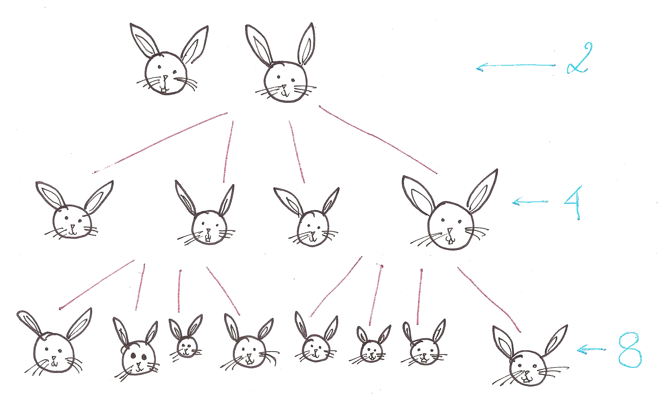
Algosaurus then remembers that game he used to love playing on the phone, which merged tiles of the same power of 2 together.
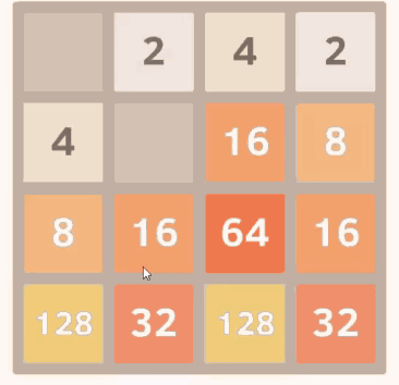
You’ve played 2048 too, right?
Let’s get some intuition using binary arithmetic now.
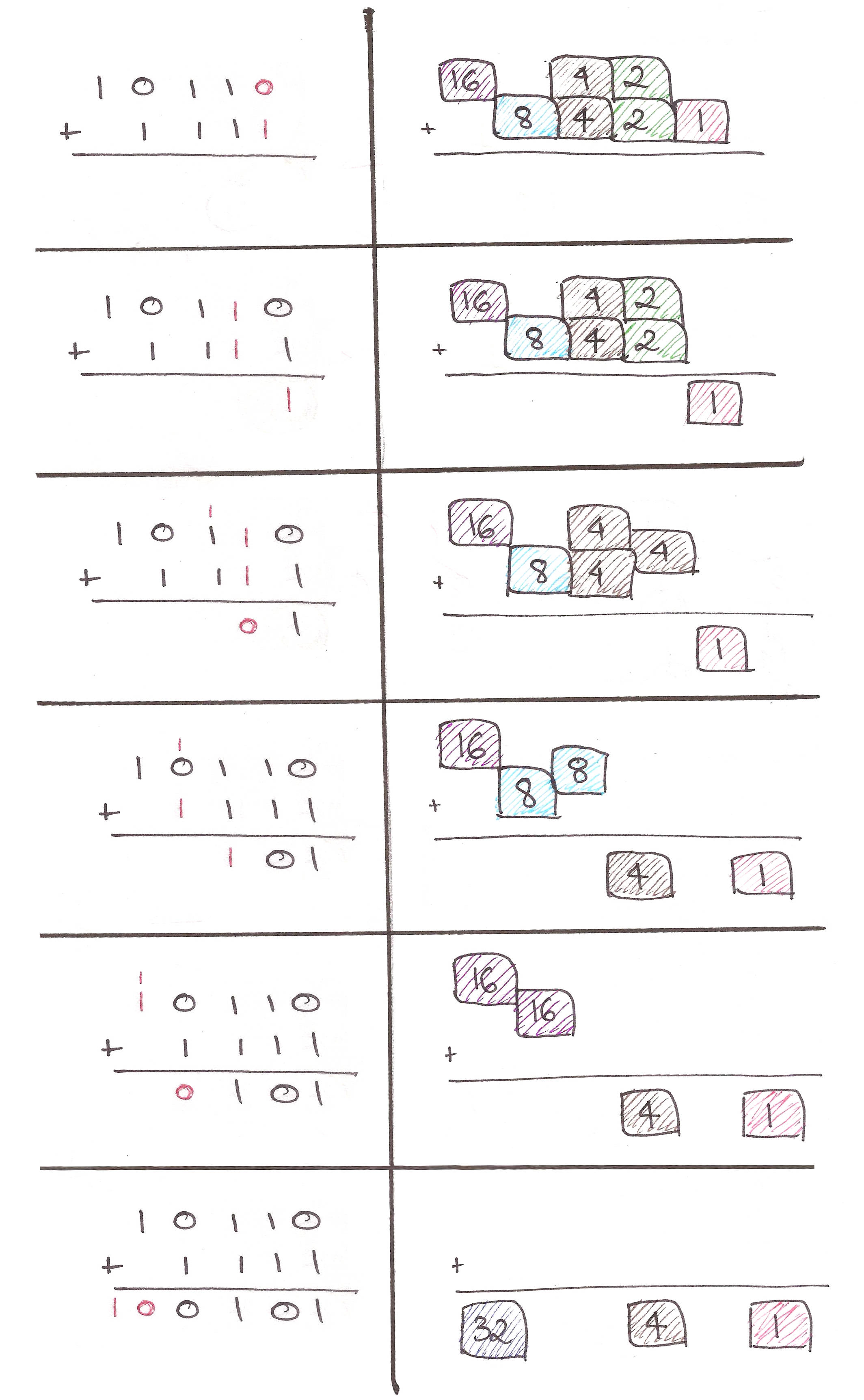
What if we could adapt this approach to store our elements in ‘packets’ whose sizes are powers of 2?
With this, we have three properties fixed:
- Sizes must be powers of two
- Can efficiently fuse packets of the same size
- Can efficiently find the minimum element of each packet
Let’s get down to deletion now.
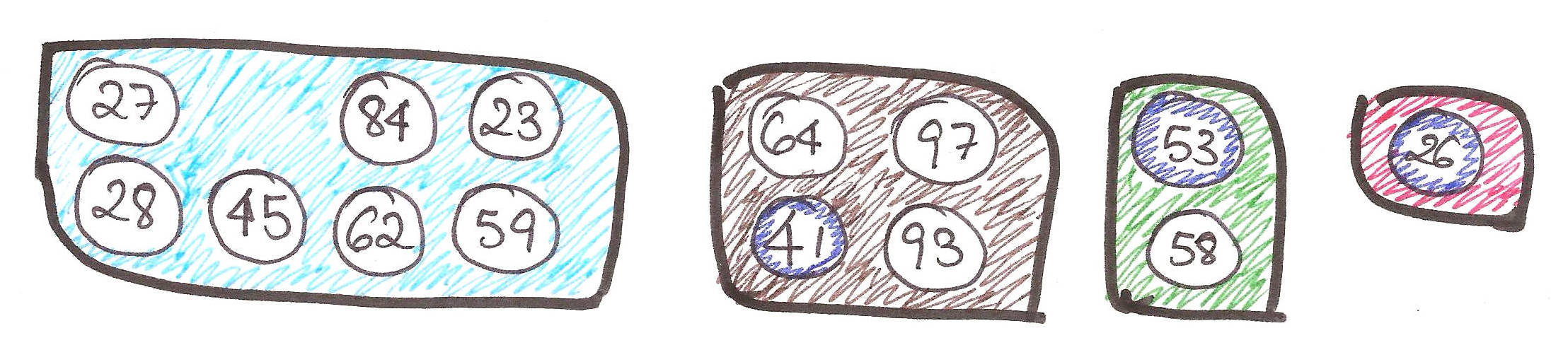
Relax Algosaurus. Remember how any number can be expressed in terms of powers of 2?
Let’s ‘fracture’ the packet from which we deleted the element.
Then put it all back together.
With that, our four properties are:
- Sizes must be powers of two
- Can efficiently fuse packets of the same size
- Can efficiently find the minimum element of each packet
- Can efficiently ‘fracture’ a packet of
 elements into similar packets of smaller powers of 2
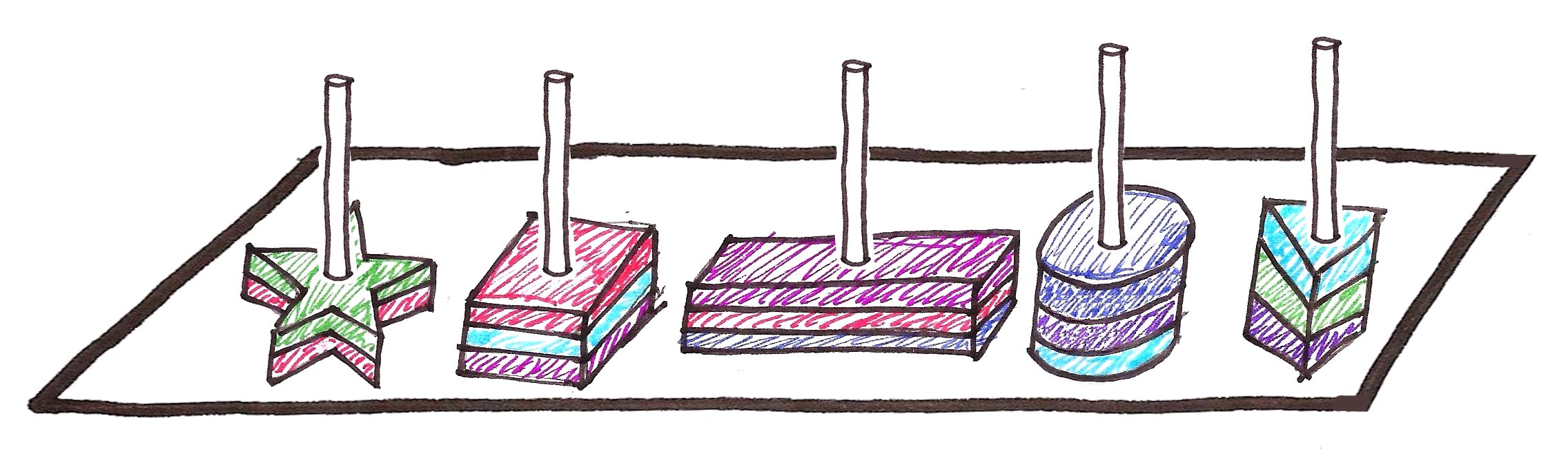
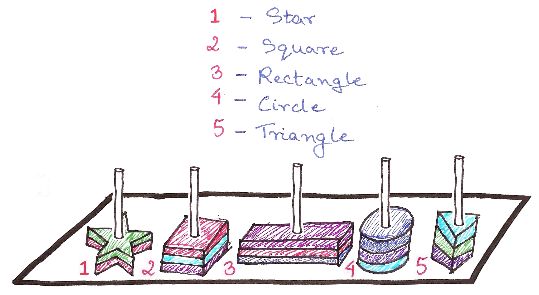
In what form should we express our packets in?
With binomial trees of course!
Quoting directly from the slides referenced in the Acknowledgements:
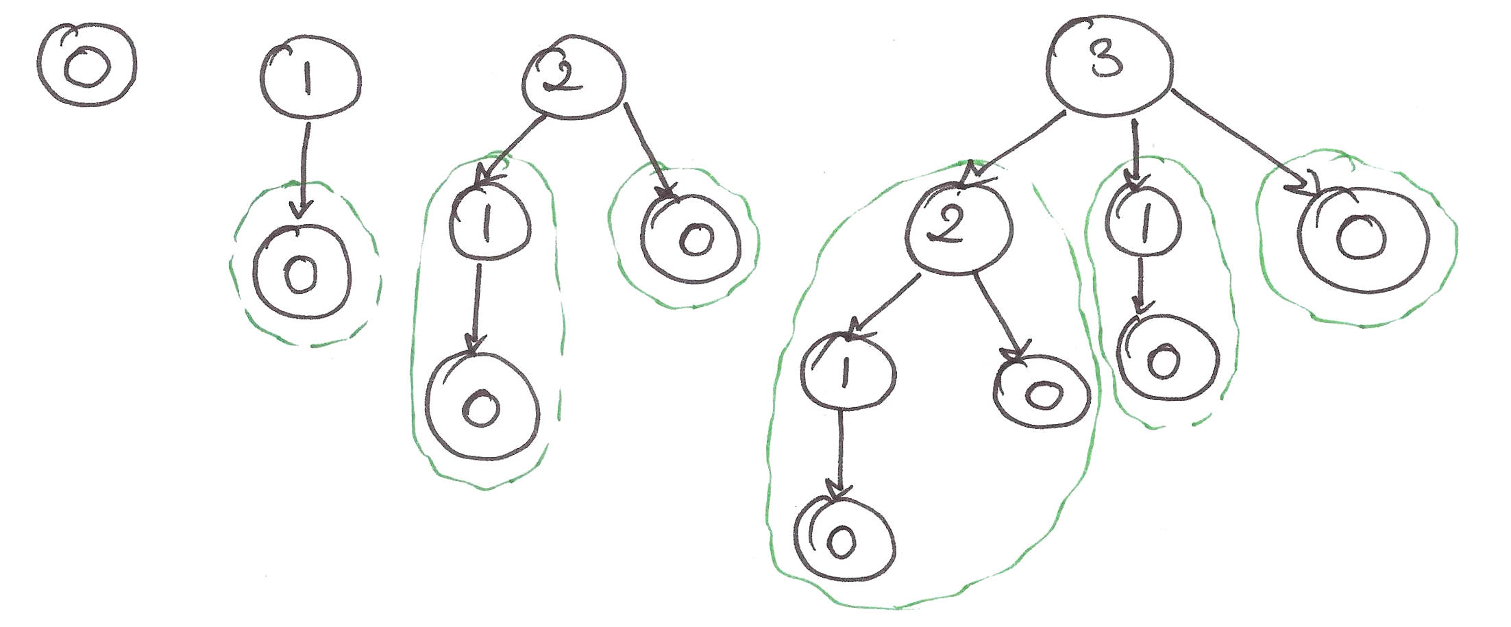
“A binomial tree of order k is a type of tree recursively defined as follows:
A binomial tree of order k is a single node whose children are binomial trees of order 0, 1, 2, …, k – 1.”
Let’s apply the heap property to the binomial trees.
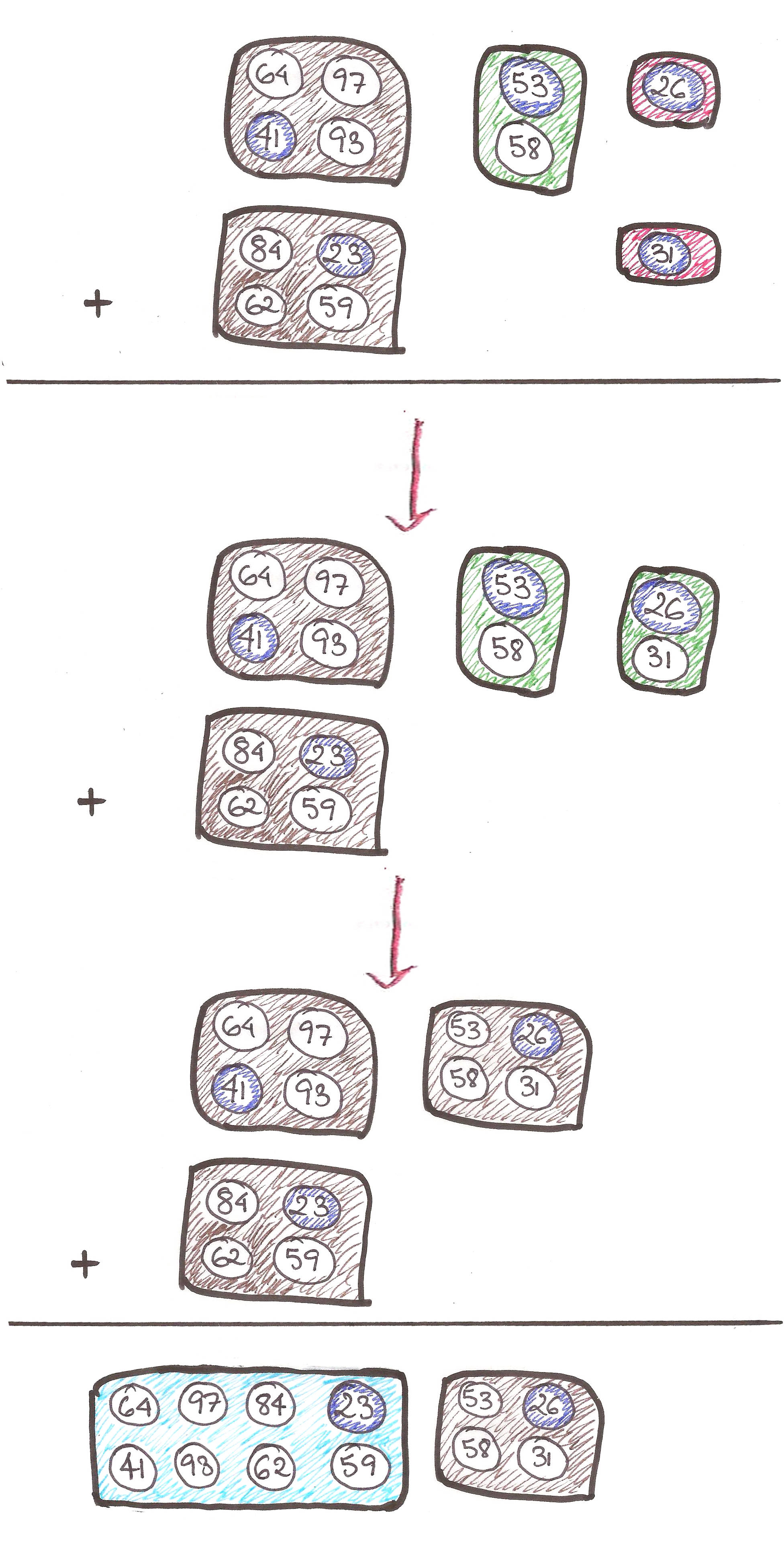
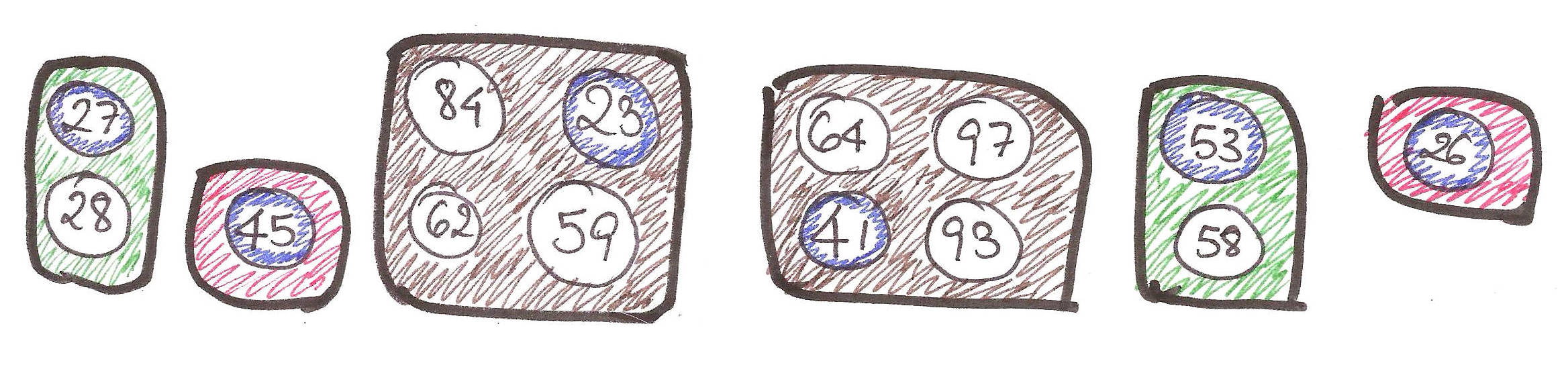
A binomial heap is basically a forest of heap-ordered binomial trees. Now, let’s check whether our binomial trees adhere to the 4 properties we set earlier.
- Sizes must be powers of two – Pretty obvious.
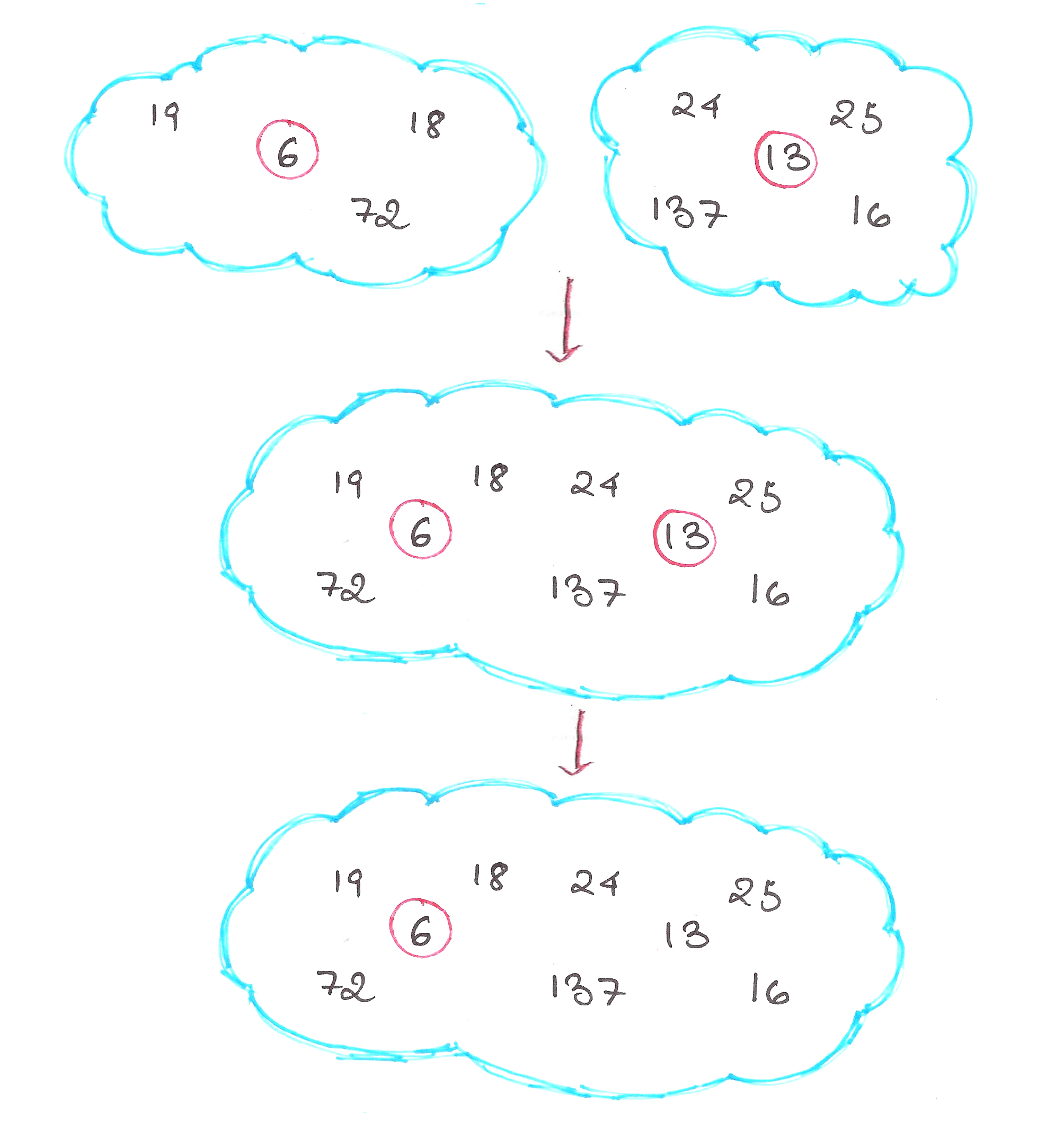
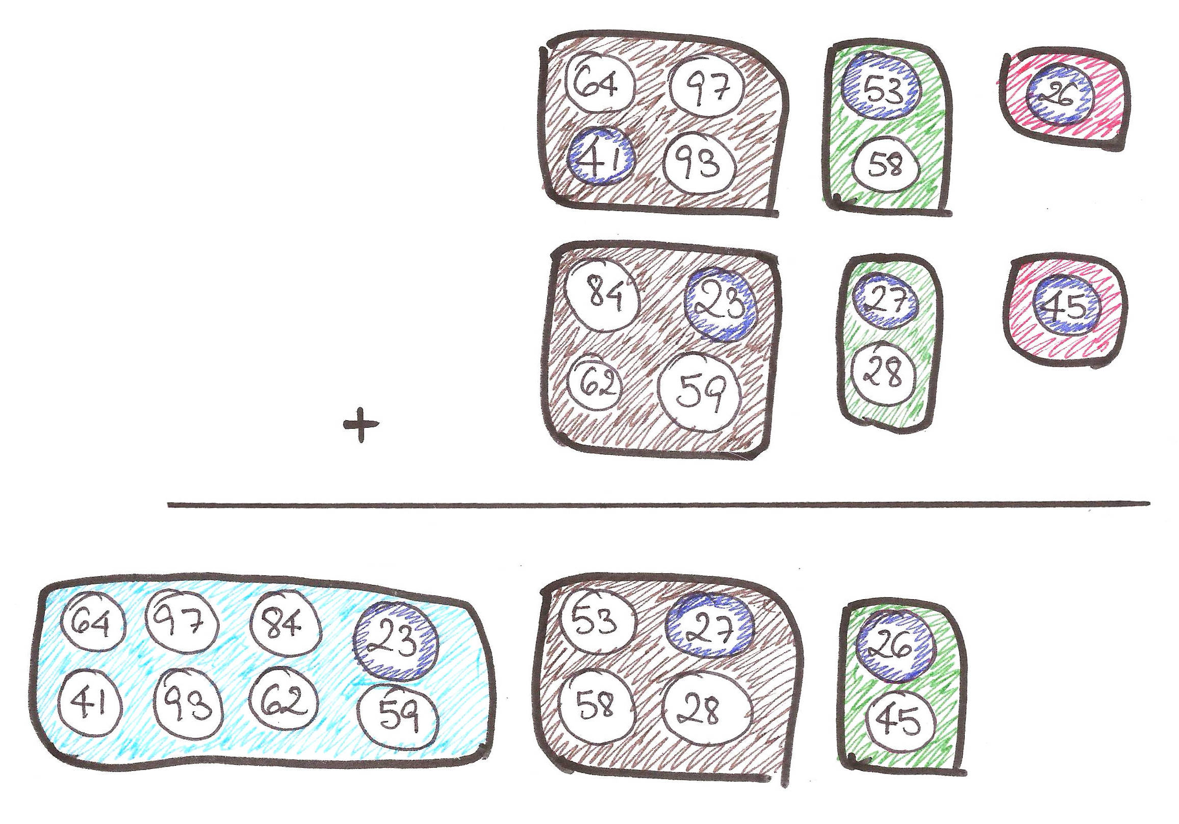
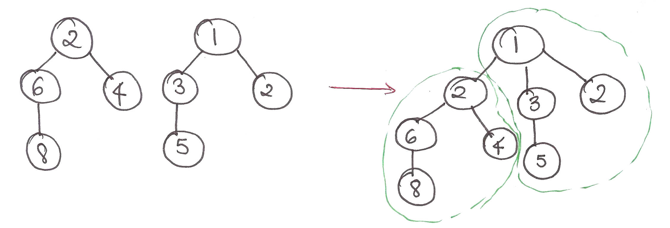
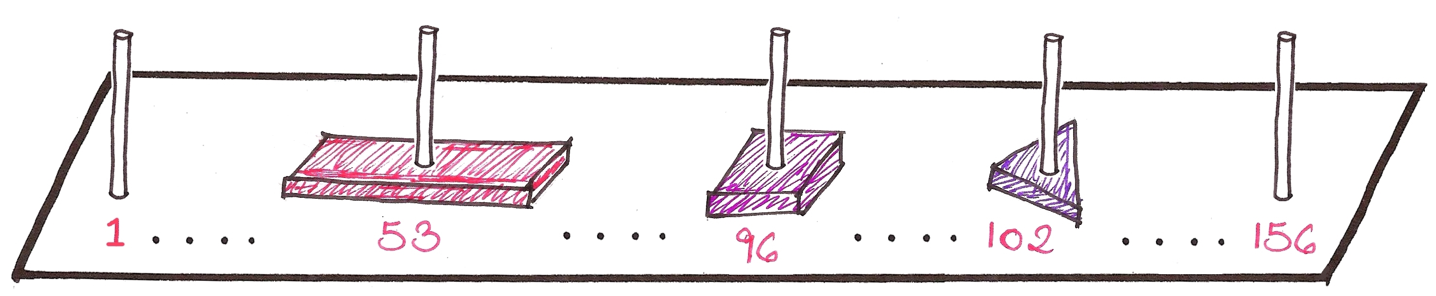
- Can efficiently fuse packets of the same size – As shown below, it’s a trivial operation!
- Can efficiently find the minimum element of each packet – Each tree has a pointer to its minimum element, so it can be retrieved in
 time.
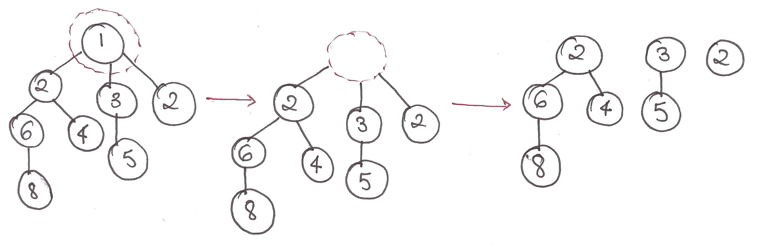
time. - Can efficiently ‘fracture’ a packet of elements into similar packets of smaller powers of 2
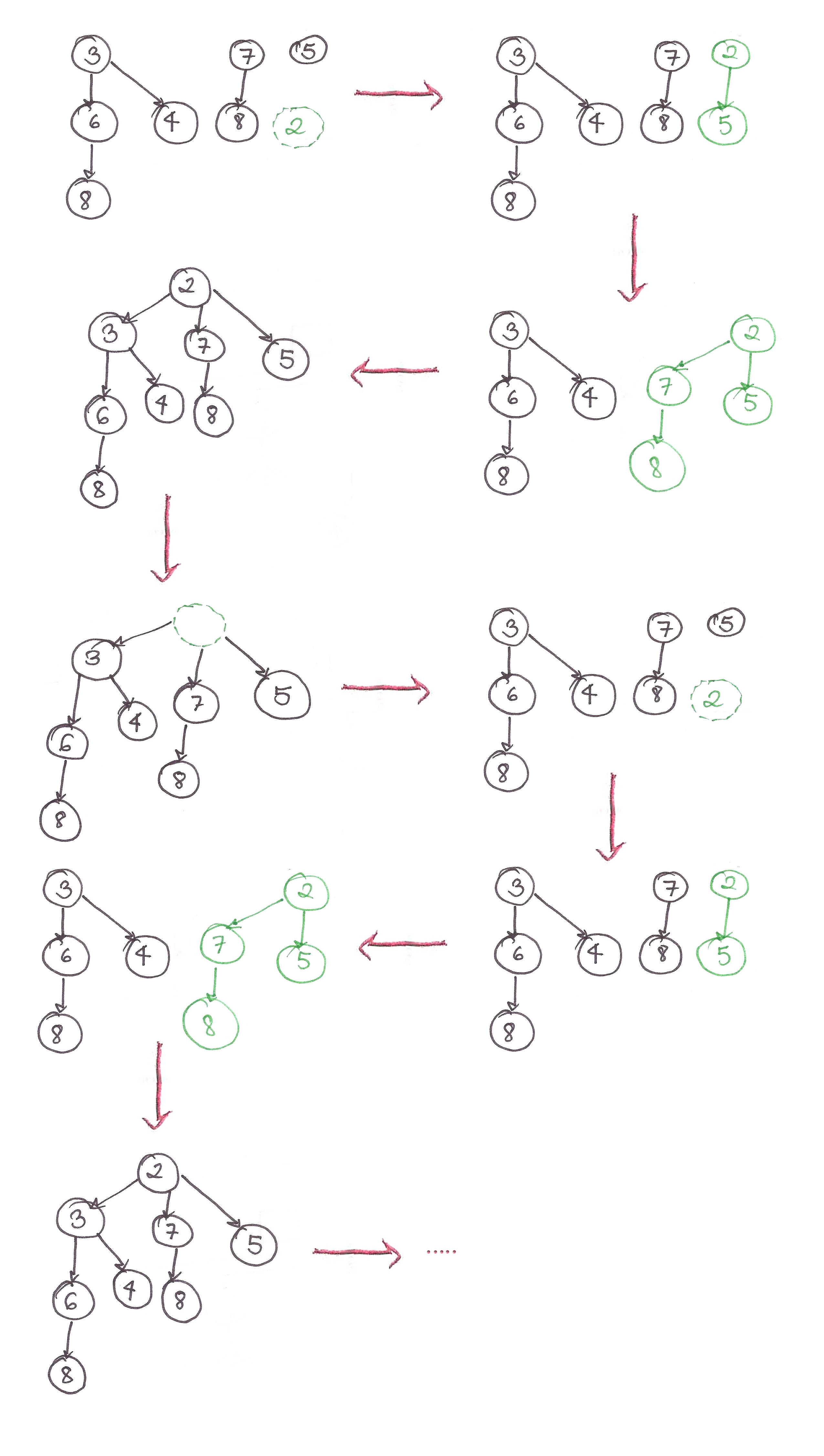
Since we’ve finally got an intuitive understanding of merging and deletion for the ‘packets’, let’s step through doing so in Binomial Heaps.
insert():
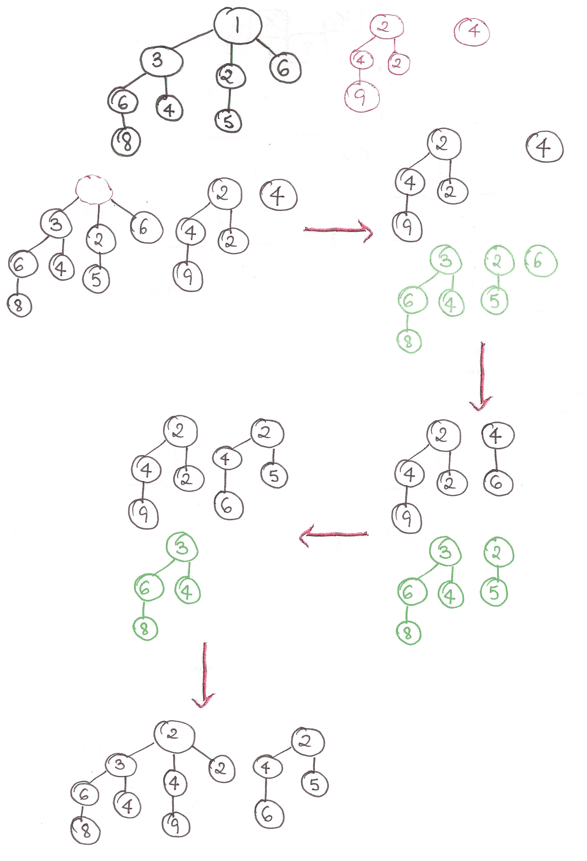
extractMin():
For now, I’m just going to say that the amortized time of insertion into a binomial heap is . Feel free to take my word, or check them out in the slides given in the Acknowledgements.
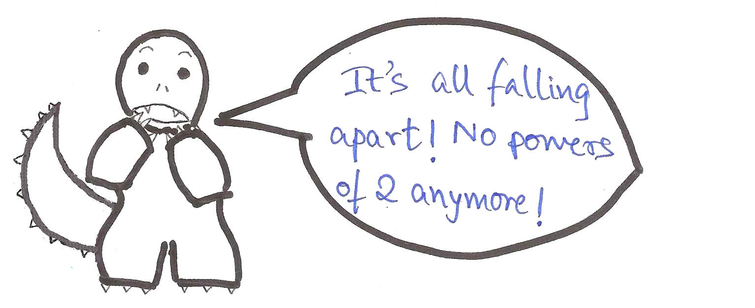
But we still have a couple of problems…
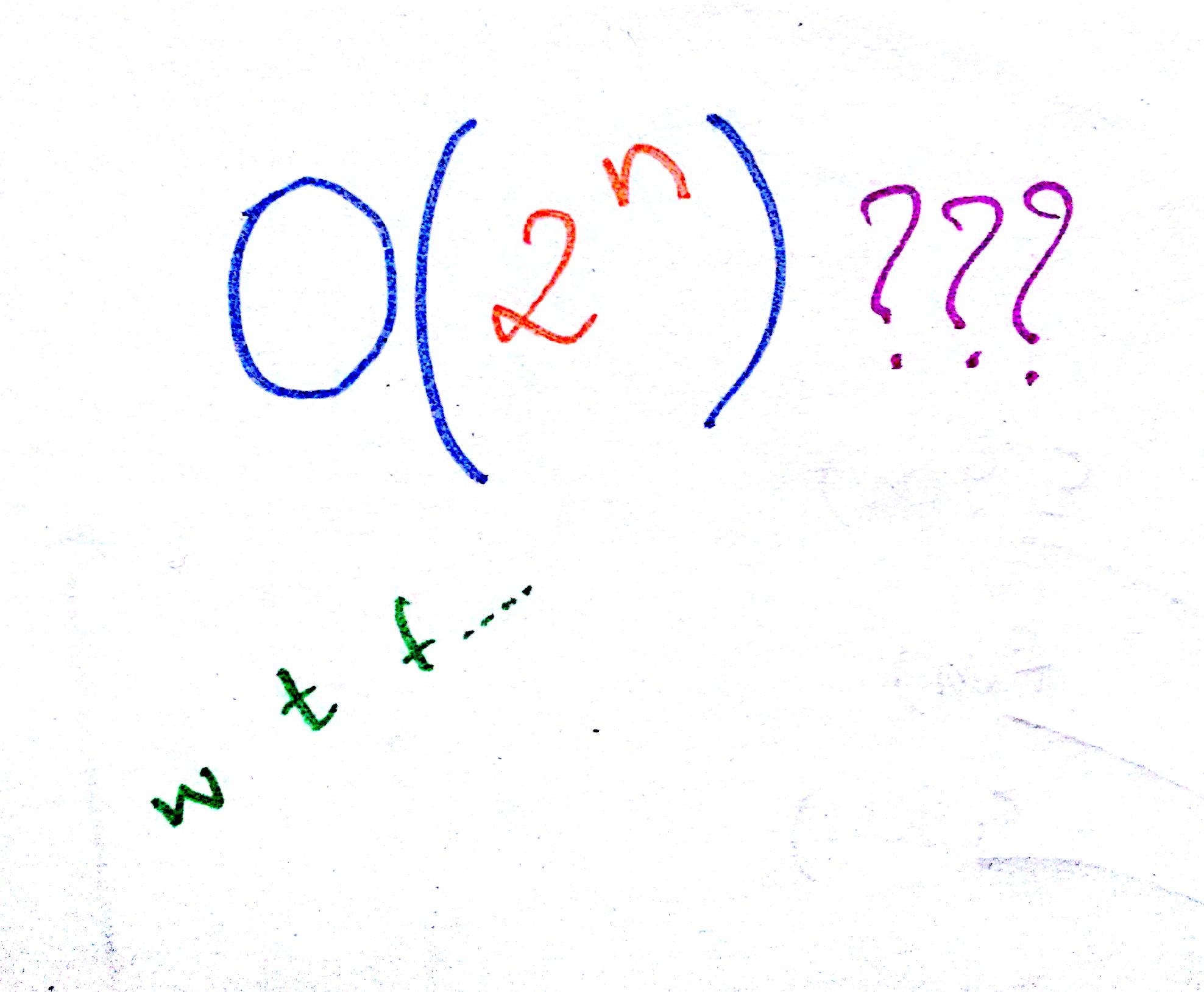
When we intermix insert() and extractMin(), we force expensive insertions to happen repeatedly, wrecking our amortized time for insertion from to , because we have to merge  binomial trees together at the same time.
Hmm. How do we make the speed of our insertion operations independent of whether we do deletions in the middle?
In Bengali we have a saying, “If you don’t have a head, you won’t have a headache”.
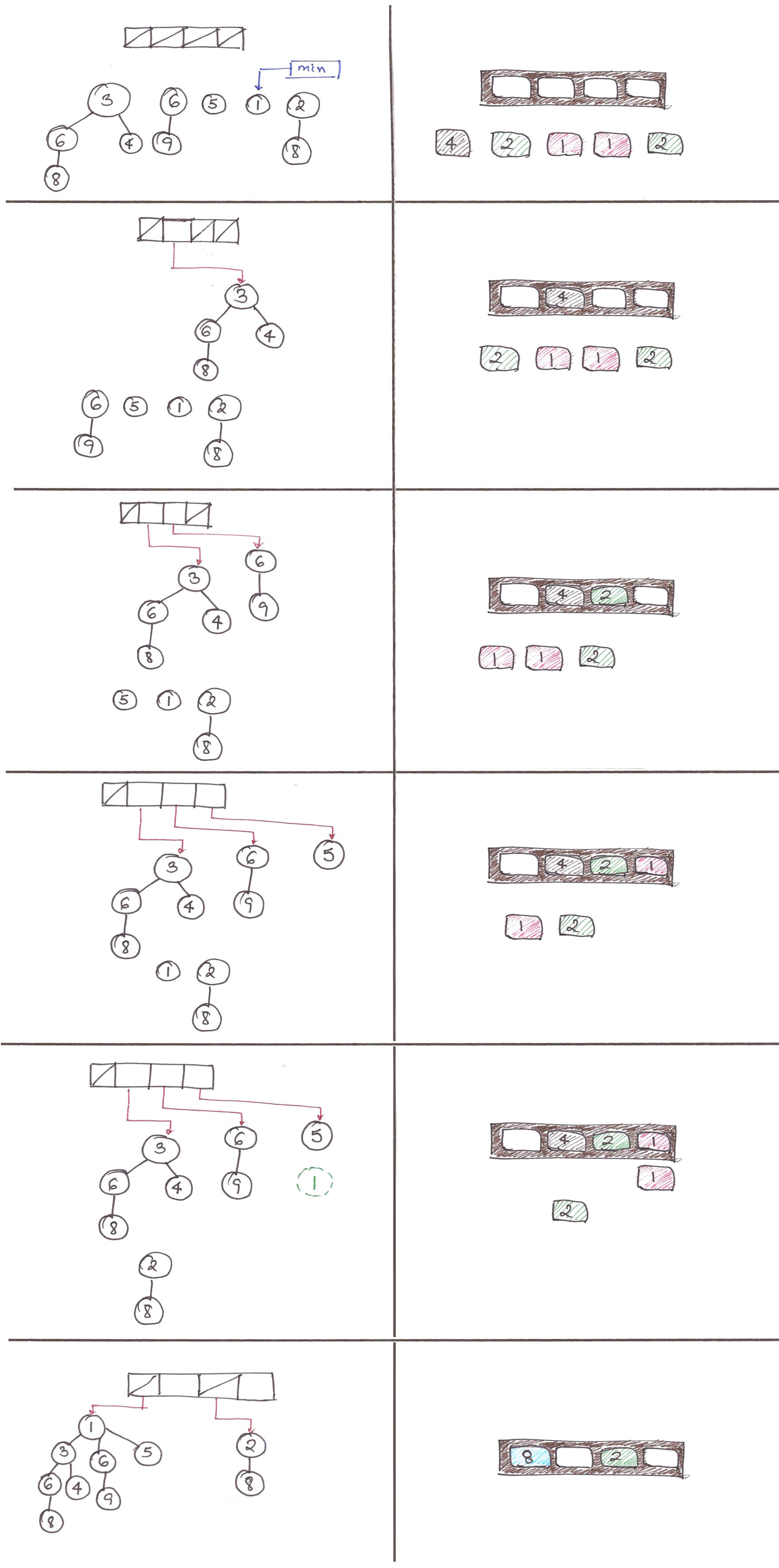
What if we just don’t merge the binomial trees together, avoiding the step altogether?
That is, just add the isolated, unmerged binomial tree to the forest with every insertion and do nothing else.
We’ll only coalesce the trees together when we call extractMin(), only when we need to. The number of trees required to coalesce all the disjoint trees, is , just like the number of bits required to represent a decimal number  , is .
We can’t just ‘merge’ all the mini-heaps together because the ‘merge’ operation assumes that all the trees in the binomial heap are in ascending order, and that isn’t the case here.
Let’s go back to our 2048-analogy for some intuition.
And we’re done!
Here are the final amortized complexities of our ‘lazy’ binomial heap:
insert():
merge():
findMin():
extractMin():
I’m not proving them here, in interest of keeping this proof-free. Feel free to check them out in the slides given in the Acknowledgements.
This concludes my article on Binomial Heaps. Although this may not have been as fun as my other articles, I hope it managed to demystify Binomial Heaps for you.
Acknowledgements:
This article simply wouldn’t have been possible without this series of slides CS166 from Stanford. These slides were the template for my article, so full props to them.
http://web.stanford.edu/class/archive/cs/cs166/cs166.1146/lectures/06/Slides06.pdf


 , where
  by default, because we really like binary stuff.
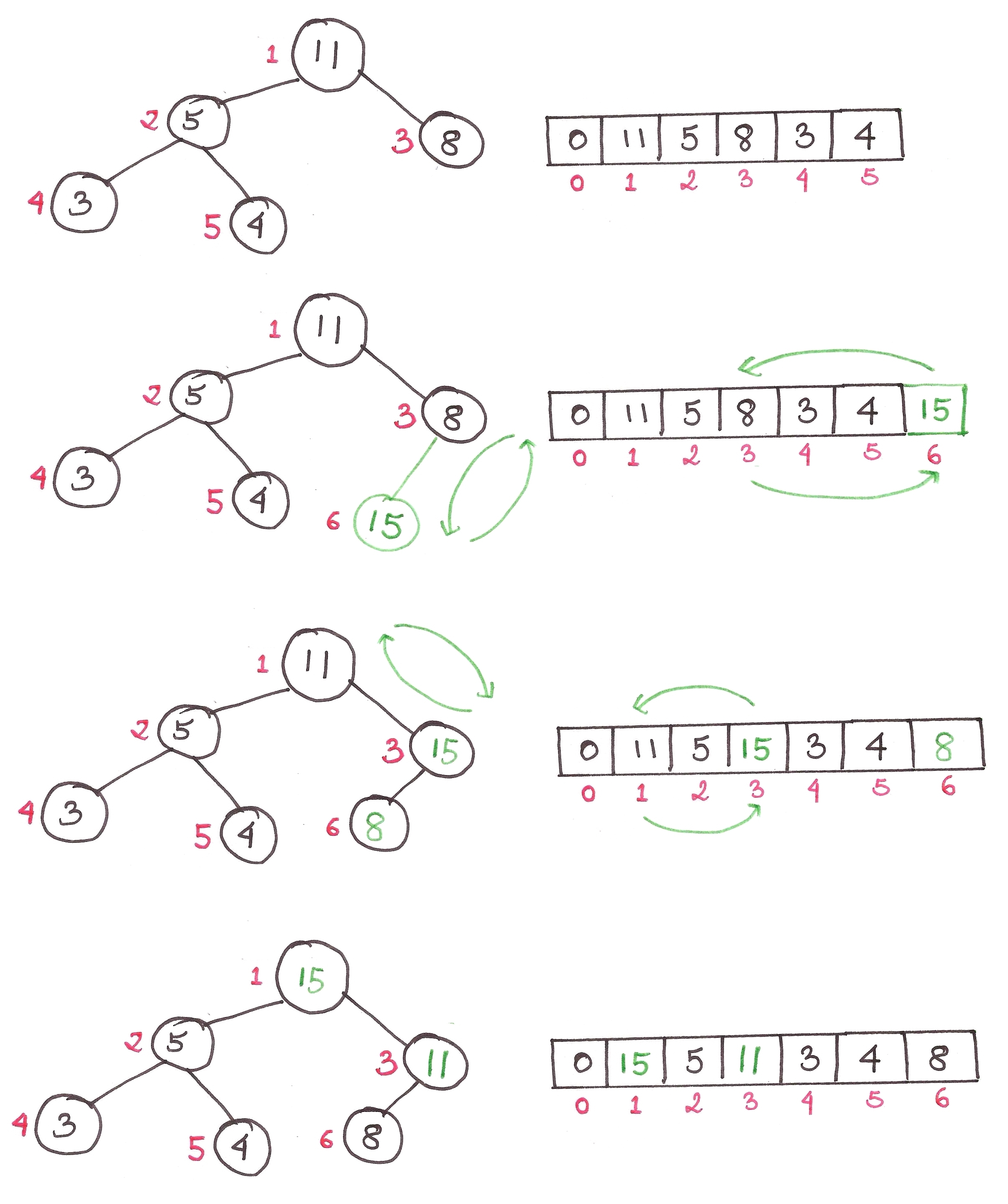
 .
.
 because of an
  element back to the 1st one.
 complexity and it’s beyond the scope of this article to prove why. Just understand that any element past the halfway point in a binary tree, will have no children and that most of the ‘sub-heaps’ formed will be of height less than
 complexities, Heapsort runs in


 to be true for now.
 is true.


 we take.