Prerequisites:

• Logical progression of thought
• Some mathematical aptitude
• Basic knowledge of functions

Recursion is possibly one of the most challenging concepts in Computer Science to get the hang of, and something which has fascinated me for a very long time. Sure, we all know the textbook definition:

“Recursion is a method where the solution to a problem depends on the solutions to smaller instances of the same problem.”

But it still takes an “Aha! Moment” to get an intuitive grasp on it, which is why I’ll finally take a stab at it.

As usual, we have three levels, so switch to them as you see fit:

• Introduction
• Apprenticeship
• Mastery

---

Algosaurus coincidentally happens to be part of an obscure death metal band you’ve never heard of. He goes to a concert venue with a poorly-designed audio system and starts off with his smash-hit song “Rock Tore My World Apart”. He growls into the mic as he descends into the chorus and…

…is rudely interrupted by a loud screeching sound from the amplifier.
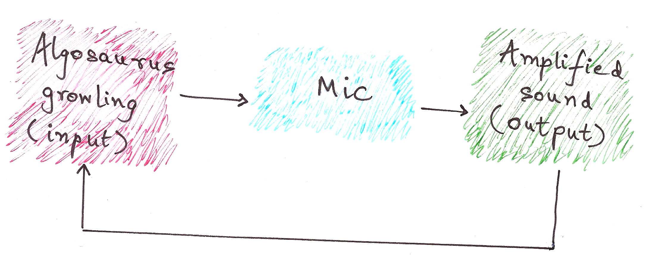
What just happened was a feedback loop. While Algosaurus was singing (growling?) his heart out, his mic picked up the output of the surrounding amplifiers, and fed it right back into the input.
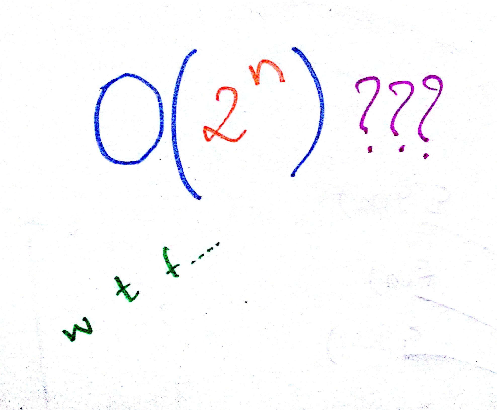
Although the above example doesn’t reduce to a meaningful output, rather it results in a stack overflow (the screeching sound), this is the essential idea of recursion.
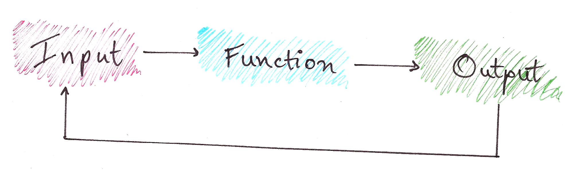In recursion, we have:

Problem
|
Sub-problem (which is Problem with a smaller input)
|
Base Case (a Problem with a constant output)

Confused by the jargon?
So was I.

---

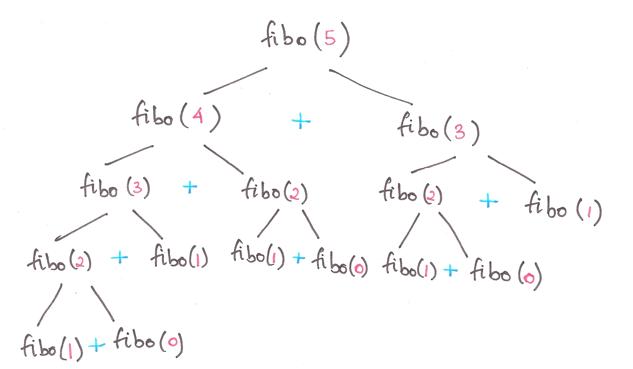
No article on recursion is complete without talking about Fibonacci Numbers.

Fibonacci series: 0, 1, 1, 2, 3, 5, 8, 13, 21…

You’ll notice that the nth Fibonacci number, after n = 0 and n = 1, is the sum of the previous two Fibonacci numbers.

Namely,

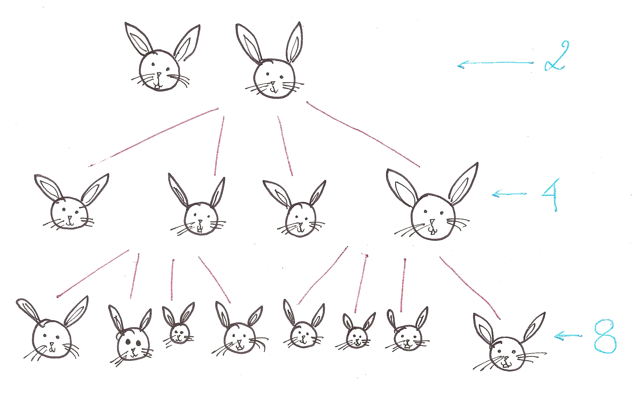
Notice how this is a recursive definition? Let’s break it down into a recursion tree.

So, let’s define Fibonacci numbers in terms of Problems and Base Cases.

Problem: 
|
Sub-problem(s): 
|
Constant Base Case: 

This is also known as the divide-and-conquer paradigm of algorithms, where we segregate a problem into smaller sub-problems, and finally into a simple base case.

Final code for Fibonacci numbers?

def fibo(n):
    if n == 0:
        result = 0 #Base case
    elif n == 1:
        result = 1 #Base case
    else:
        result = fibo(n-1) + fibo(n-2) #Feeding the 'output' right back into the input function
    return result

Lo and behold, you just learnt recursion.

---

Let’s take another classic example to hit the point home.

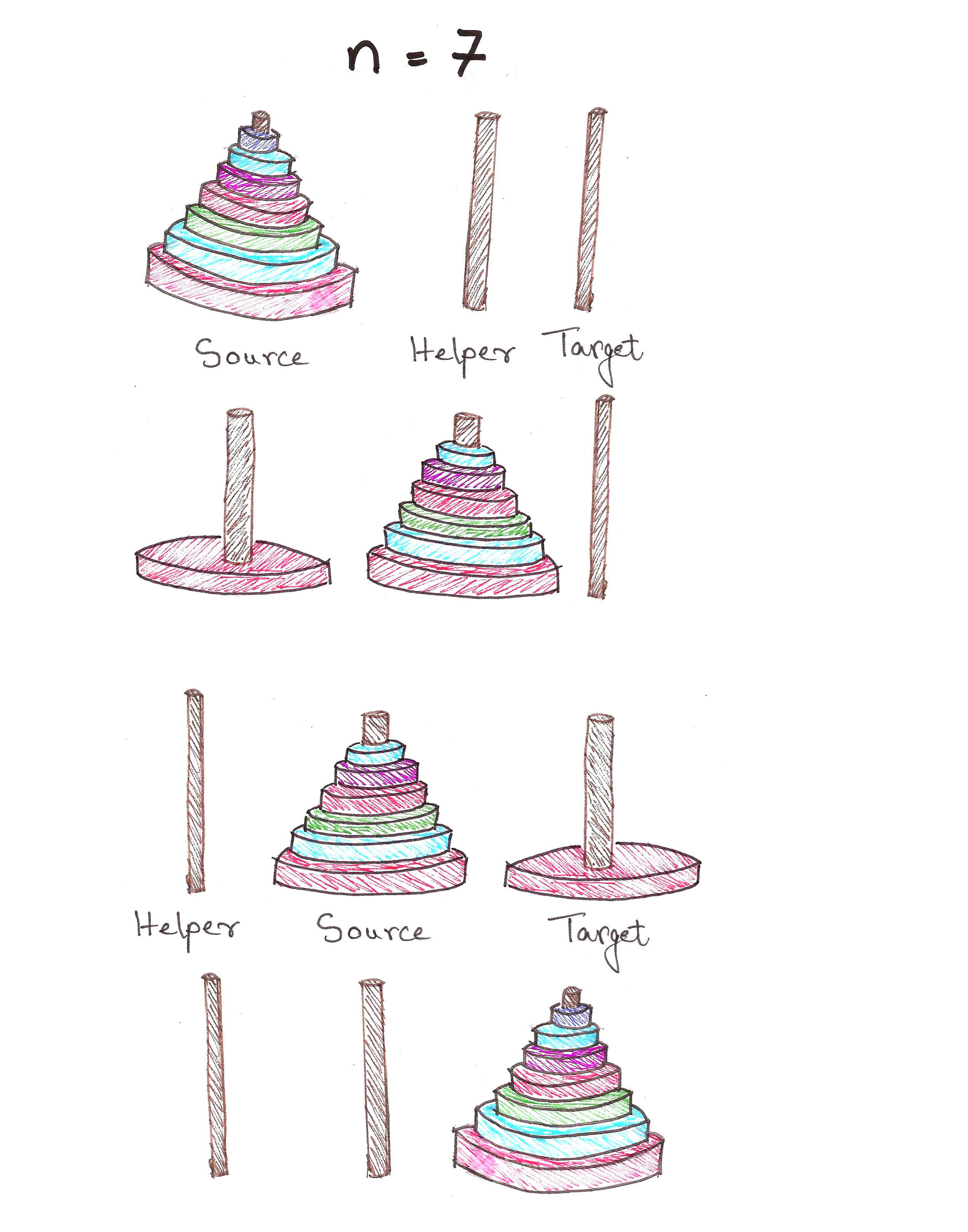
Once upon a time, in the Cretaceous Era, there lived a family of Algosauri in a land far, far away. Baby Algosaurus had a toy with 3 rods and 7 discs.

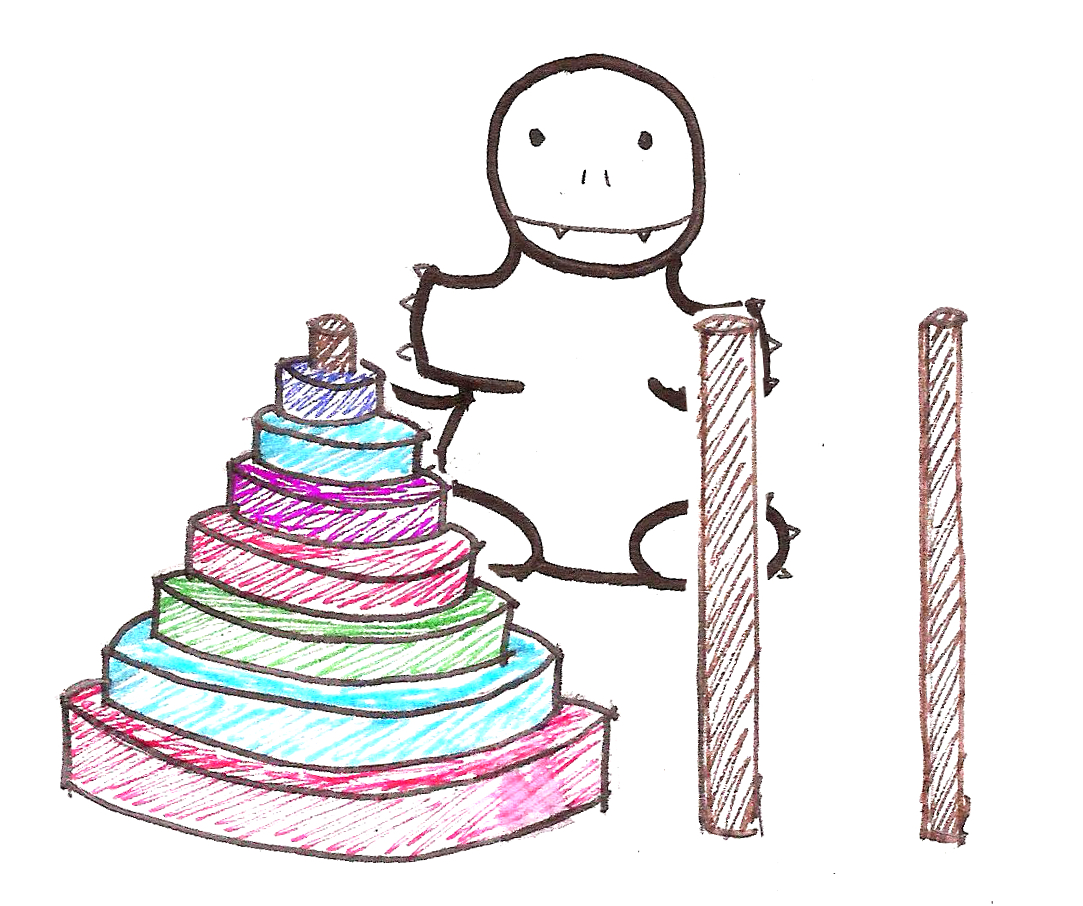
His Dad challenged him to a game, where the objective was to transfer all the discs to another rod, obeying the following rules:

1. Only one disk may be moved at a time.
2. Only the uppermost disk from one rod can be moved at once.
3. It can be put on another rod, only if that rod is empty or if the uppermost disk of that rod is larger than the disc being moved.

How did Baby Algosaurus do it?

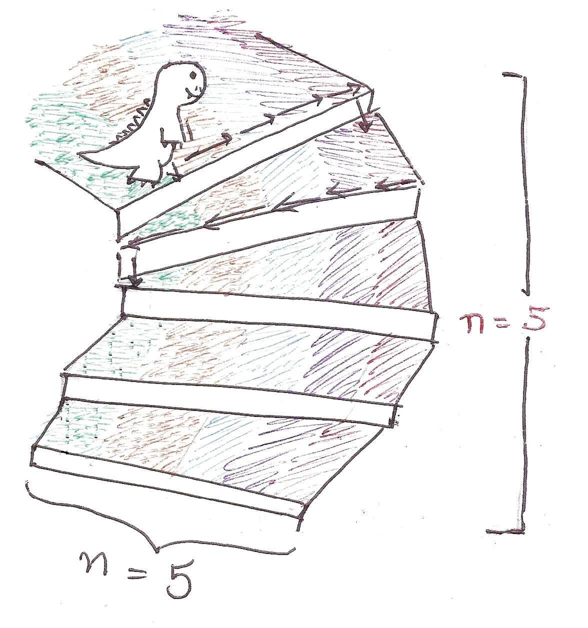
Let’s assume there to be n number of discs, and we’ll be moving the tower from source to target using the helper rod:

For n = 1:
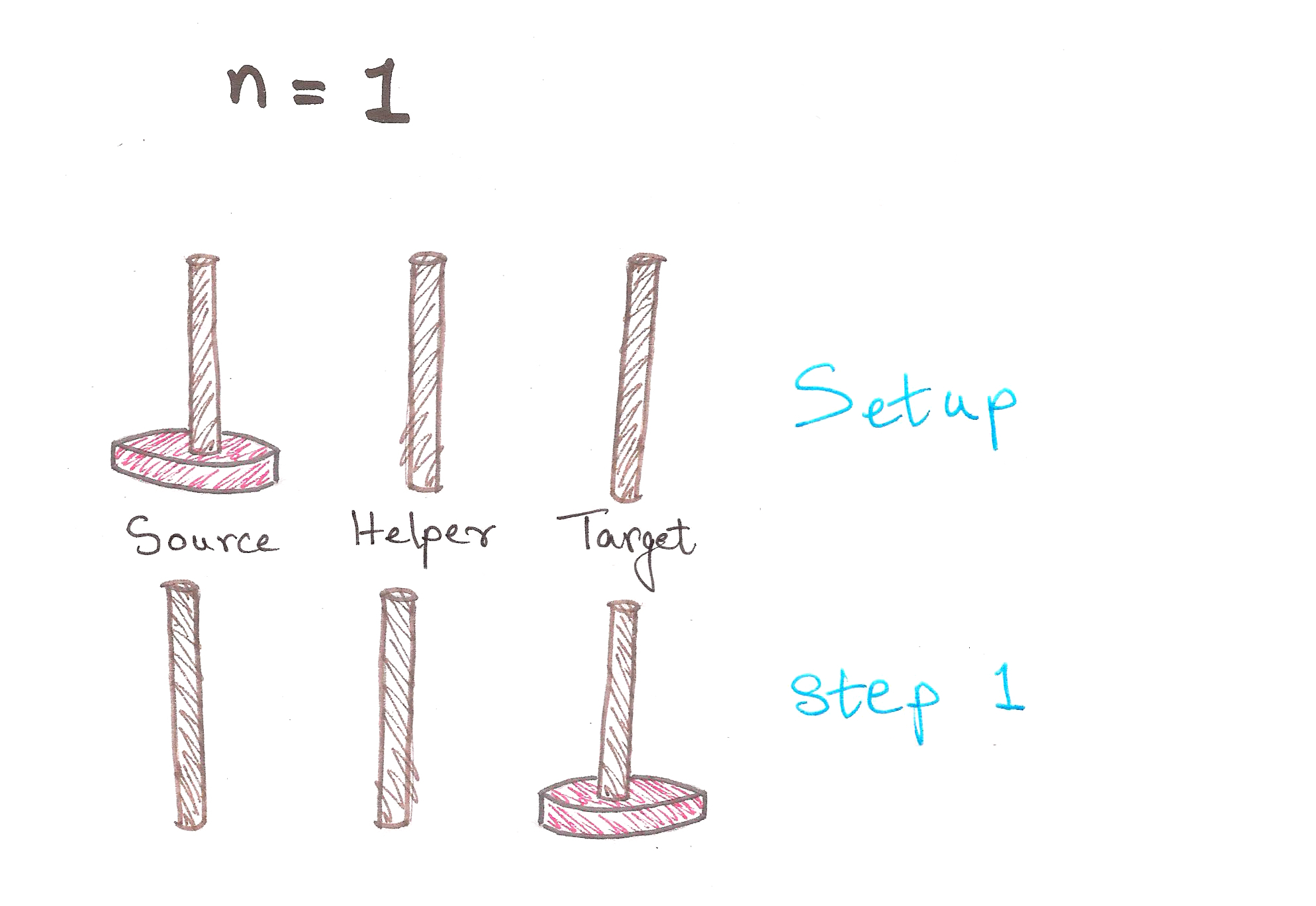1 step. Easy enough.

For n = 2:

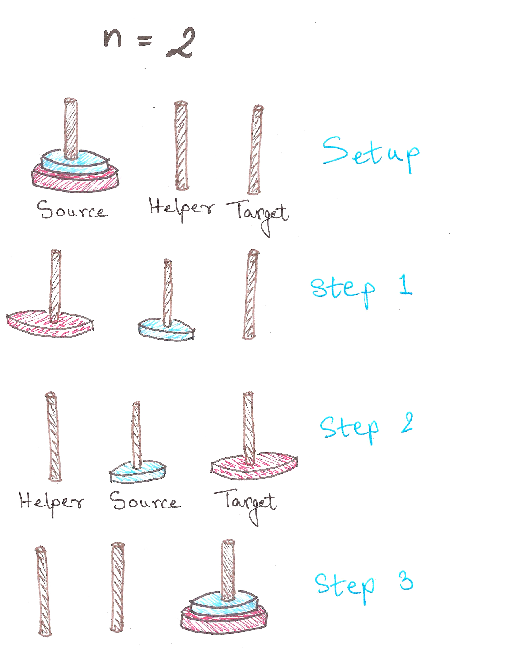
3 steps. We’re moving along now.
In Step 1, notice how after we shift the 1st disc to Helper, we have a tower of n – 1 = 1 disc, on Helper.

For n = 3:

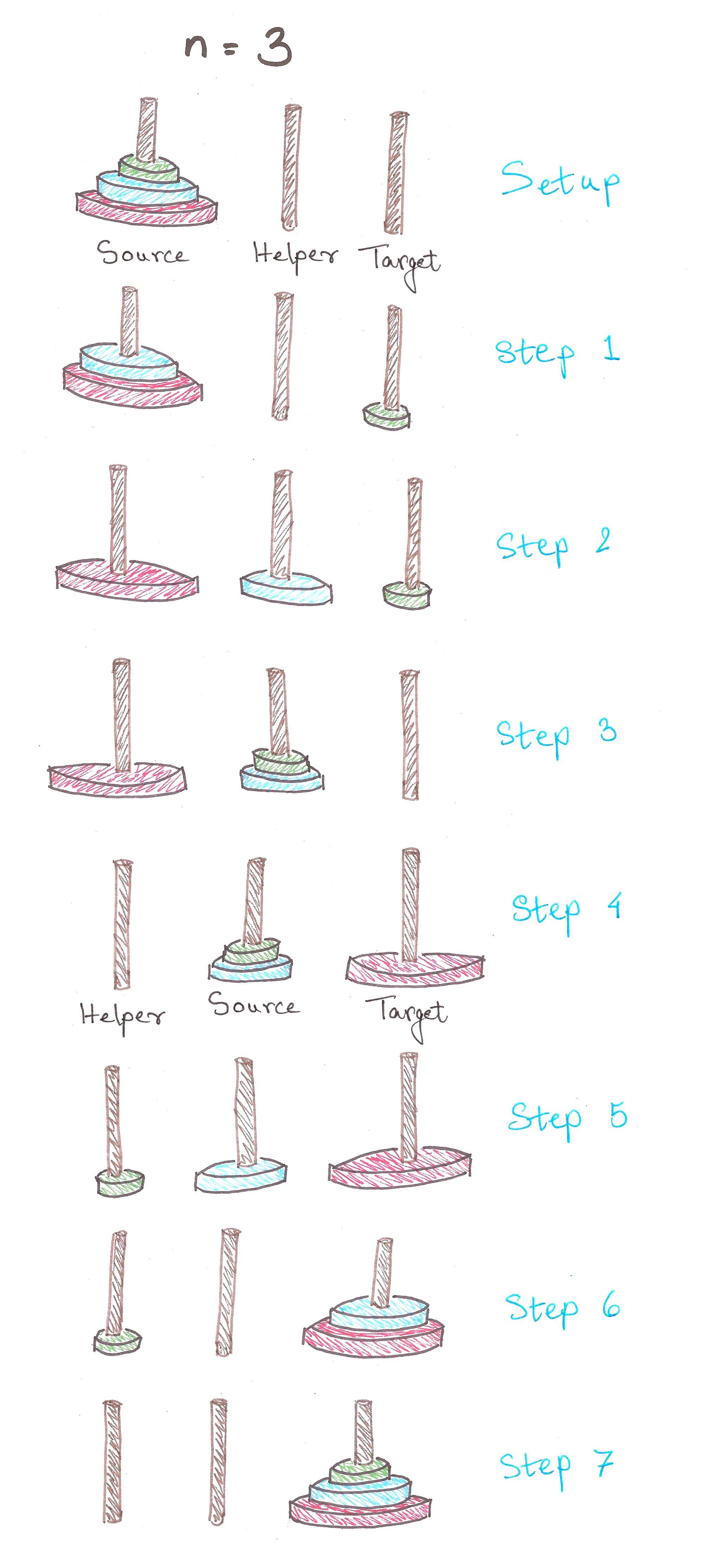
And we’re done in 7 steps!
Observe that in Step 3, we have a tower of n – 1 = 2 discs, on Helper now. Notice anything similar to the previous case?

In case you haven’t noticed…

In fact, we can prove by mathematical induction, that the least number of moves required to solve a tower of n discs is:

Click here if you’d like to see the proof for yourself.

---

Back? Good.

We now need to solve the problem for n = 7. We can of course, figure it out by hand as above, but what’re we learning recursion for then?

A quick recap of the divide-and-conquer method:

Problem
|
Sub-problem (which is a Problem with a smaller input)
|
Base Case (a Problem with a constant output)

So here, in the Tower of Hanoi problem (yeah, that’s the official name), we have:

The general rule for moving towers:
Problem: Moving tower of n discs from Source to Target
|
Sub-Problem: Moving tower of n – 1 discs from Source to Helper, then moving last disc to Target
|
Base Case: Moving tower of n = 1

Great. Let’s finally translate this into code.

def hanoi(n, source, helper, target):
    if n > 0:
        hanoi(n - 1, source, target, helper)    #moving tower of size n - 1 to helper:
        #moving disk from source peg to target peg
        if source:    #checks whether source is empty or not
            target.append(source.pop())    #appends the last disc from source, to target
        hanoi(n - 1, helper, source, target)    #moving tower of size n-1 from helper to target
        
source = [4,3,2,1]
target = []
helper = []
hanoi(len(source),source,helper,target)

print source, helper, target

Feel free to go through this entire section once more to digest it, because it’s pretty mentally intensive if you aren’t yet used to thinking this way.

---

Proof by induction:

The base cases for this problem are pretty simple…

Let’s assume to be true for now.

To prove: is true.

So we have,

Hence proved. Click here to go back up.

---

Self-similarity is symmetry across scale. It implies recursion, pattern inside of pattern. Monstrous shapes like the Koch Curve display self-similarity because they look exactly the same, even under high magnification. Self-similarity is an easily recognizable quality. It’s images are everywhere in the culture: in the infinitely deep reflection of a person standing between two mirrors, or in the cartoon notion of a fish eating a smaller fish eating a smaller fish eating a smaller fish.

– Chaos – The Amazing Science of the Unpredictable, James Gleick

In 1976, a biologist named Robert May published a seminal paper on the population of animals. This paper would soon create a storm, and not just in biology.

Let’s take a look at what it was all about.

May proposed that variation in population of animals could be modeled by a simple equation, formally called the logistic equation:

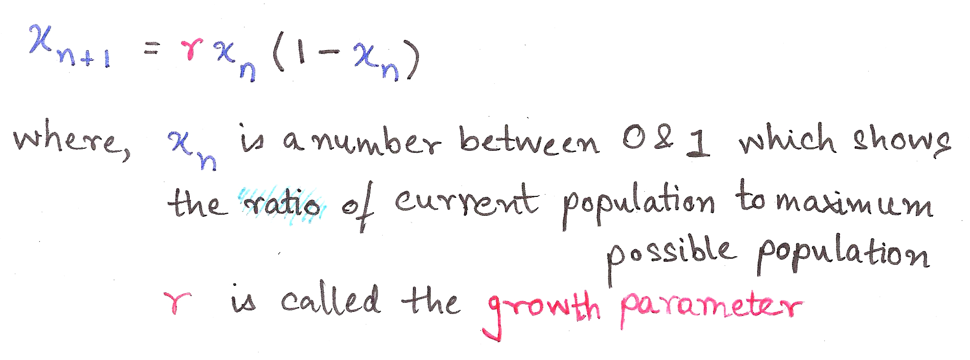
This is a recurrence relation, an equation which recursively spits out values as a function of its previous values, ie. takes the output and shoves it back into the input.

It’s such a cute equation, isn’t it? Who’d guess that its interpretation could transform into *this*…

This is called a bifurcation diagram, and is also a kind of fractal. It shows the values the population of the species evaluates to finally (as time tends to infinity), depending on the value of r, the growth parameter.

Let’s dissect this.

r between 0 and 1 – Population dies out
r between 1 and 3 – Population converges to a single value
r between 3 and 3.44 – Population oscillates between two values
r between 3.44 and 3.54 – Oscillates between four values
r between 3.54 and 3.56 – Oscillates between 8 values

All of the above are pretty much independent of initial conditions, ie. the initial we take.

What about 3.56 onward?
Chaos.

Slight differences in initial conditions result in dramatic changes in population, with no particular order. (In science-y language, ‘Extreme sensitivity to initial conditions’)

This particular paper was path-breaking because it showed how Chaos Theory and fractals aren’t obscure theoretical constructs; they’re things which explain real-life phenomena and its glorious imperfections.

This is a bit beyond the scope of this article, but it goes to show how wide-ranging a role does Recursion play, not just in computer science, but in nature itself.

---

I hope you now have enough a grasp on thinking recursively to understand algorithms like Quick Sort and Merge Sort, and attempt a few basic ad-hoc problems from Codechef et al.

If you are just as fascinated as I am about recursion, then you might enjoy reading about the following:
Fractals
Chaos Theory
Infinite Series and Loops
Feedback loops in Op-amps (they’re an essential part of electronics)

I plan on writing more about the above topics, so do subscribe to Algosaurus for updates.

If you liked this guide, want to insult me, or if you want to talk about dinosaurs or whatever, shoot me a mail at rawrr@algosaur.us

Acknowledgements:
http://www.python-course.eu/towers_of_hanoi.php
https://en.wikipedia.org/wiki/Logistic_map

Prerequisites:

• Exponentiation
• Basic algebra
• Functions and asymptotes
• Prior knowledge of Insertion Sort and other basic sorts of sorts

This post is roughly divided into three parts, so feel free to switch to either part depending on your level:

• Introduction
• Apprenticeship
• Mastery

---

Algorithmic complexity and growth of functions form the very foundation of algorithms. They give us an idea of how fast or slow an algorithm is, so you can’t go anywhere near designing and analyzing ’em without having these as tools.

Algosaurus wants to know what ‘growth of functions’ means. So he decides to get two bunnies. And the bunnies start having kids, hypothetically four per couple. Lots of them, because well, erm…

If we examine the growth of bunnies, we find that it grows at the rate of 2^n, where n is the number of generations. This isn’t very good news for Algosaurus, because despite bunnies being cute and cuddly, there is something called having too many bunnies.

Roughly speaking, Bunny Breeding Algorithm has a complexity of O(2^n).

This is because the number of bunnies in next generation (the output) grows exponentially with respect to the number of bunnies we started with (the input).

Let’s dissect this.

“Order of growth of the running time of an algorithm gives a simple characterization of the algorithm’s efficiency and also allow us to compare the relative performance of alternative algorithms”.

– Holy Gospel of CLRS

Damn, that’s a mouthful.

Imagine Algosaurus is descending a very odd staircase with n stairs. To descend each stair, he has to walk n tiles horizontally, and only then he can step down.

So for each stair, he has to walk n tiles. Therefore, for n stairs, he must walk n^2 tiles.

def weirdStairs(nofStairs):
    steps = 0
    for i in range(0, nofStairs):
        steps += nofStairs
        steps += 1
    print steps

Total time taken to walk the entire flight of stairs?

---

Similarly, let’s take the example of the Insertion Sort.

def insertionSort(list):
    for i in range(1, len(list)):                                     
        currentValue = list[i]                                         
        position = index                                

        while position > 0 and list[position - 1] > currentValue:
            list[position] = list[position - 1]
        list[position] = currentValue

Suppose the list is in descending order and every number has to be “inserted” into the right place, ie. each line of code in the loops is executed for every element.

As you go through the code, you’ll notice that for each element present in the list, it will have to iterate through the rest of elements in the list.

If n is the length of the list, the performance isn’t linearly proportional to n, it’s proportional to the square of n.

So, the worst case running time of the Insertion Sort comes out to be O(n^2), the ‘big-oh’ being part of standard notation and ‘n’ being the total number of elements in the list.

This is the worst case performance of the Insertion Sort, and usually the only kind of performance we care about.

We’ve only talked about lists with 10, maybe 100 elements. What about those with 1000, or even a million elements? Something like the total number of Facebook users?

Oh boy, then algorithmic complexity really begins to play a role.

The number of elements is so large in these cases, that only the highest power, ie. degree, of the polynomial matters, and nothing more. The rest of the terms are rendered insignificant.

The priority order for growth of functions is as follows:
Also, roughly speaking, we can estimate the complexity of an algorithm by analyzing its loop structure.

Traversing a list is an O(n) operation, so is finding the length of one. This means running time is directly proportional to the number of elements.

def traversal(list):
    for i in range(len(list)):
        print list[i]

So at this point, Algosaurus knows enough about the growth of functions to figure out whether one algorithm is faster than the other. Yaaaaay.

For a more formal treatment of complexity analysis, read on. Or maybe come back to it after a cup of tea when all this has sunk in. *Subtle plug for bookmarking this page*

---

Opening CLRS page 43, Algosaurus sees…

Let’s first talk about ‘asymptotic notation’. As you probably know, when the input of certain functions tends to infinity, the output sometimes approaches a line, but doesn’t quite touch it. This line is called an asymptote. You should care because when designing a particular algorithm or implementing one, it is important to know how it will perform with huge input sizes. You already know what big-oh notation means: it tells you the worst-case performance of an algorithm. Let’s switch to big-omega. I’ll use the last example again. Suppose our input list is sorted to begin with, ie. the best-case performance.

def insertionSort(someList):
    for i in range(1, len(someList)):                                     
        currentValue = someList[i]                                         
        position = i                                

        while position > 0 and someList[position - 1] > currentValue:
            someList[position] = someList[position - 1]
            position -= 1
        someList[position] = currentValue
    return someList

We’ll still have to traverse every element in the list to determine whether it is sorted or not, even if we don’t go into the nested while loop. The outer loop is still executed ‘n’ times in the best case scenario.

So the best case performance turns out to Ω(n).

To digest what the rest of the godforsaken symbols mean, we need some math, namely…

Functions! And graphs!

Formally speaking, we can define Θ, O, and Ω as the following.

This doesn’t really mean much, to be honest. Let’s bring out the big guns: graphs. (Plugged from page 45 of CLRS)

A few finer points. These functions are defined only when f(n) is monotonically adhering to the required constraints after n_0.

For example, for big-omega, Ω(g(n)) is formally defined only when it is less than the runtime of the function (c*g(n)) for all values greater than n_0.

a) This is for big-theta. It is sandwiched by two functions, showing that Θ(g(n)) is defined only when it is bound from the upper and the lower sides. You can’t just say it, you gotta prove it. Hard work.

b) This is for big-oh. The runtime function is always less than O(g(n)), showing that big-oh is the *upper bound* for the runtime. Actual performance won’t be worse than this.

c) For big-omega. The runtime function is always greater than Ω(g(n)), showing that big-omega is the *lower bound* for the runtime. You can’t do much better than this.

Patience Algosaurus. Here are the practical implications:

1. Big-omega is useful when you need a *lower bound* for the time, to show that an algorithm will always be slower than Ω(g(n)). Best-case performance.
Meh, sometimes used.

2. Big-oh is used when you need an *upper bound* for the time, to show that an algorithm will always be faster than O(g(n)). Worst-case performance.
Used all the time.

3. Finding big-theta is usually harder than big-oh, so big-oh is used more frequently, despite big-theta being more mathematically accurate. Math folks must find it blasphemous, but no can do.

Phew, that was a lot of theory.

---

I hope you found this informal guide to algorithmic complexity analysis useful. If you liked it, want to insult me, or if you want to talk about dinosaurs or whatever, shoot me a mail at rawrr@algosaur.us

Acknowledgements:
Introduction to Algorithms – Cormen, Leiserson, Rivest, and Stein (pages 43 – 64)
Algorithms – Dasgupta, Papadimitrou, and Vazirani (For the priority order)
Numbers: The Key to the Universe – Kjartan Poskitt (Bunny example inspired by this book)